C Caution with classes
Care must be given to processing raster layers that contain class values (like in the case of our water layer where 1 = “water” and 0 = “land”) instead of continuous numerical values (e.g. the raster layers with bioclimatic variables).
In order to demonstrate this, let’s first load the water raster again and explore it:
### Load and explore the water raster
water <- rast("data/water.tif")
water
## class       : SpatRaster
## dimensions  : 108, 264, 1  (nrow, ncol, nlyr)
## resolution  : 0.08333333, 0.08333333  (x, y)
## extent      : -3, 19, 46, 55  (xmin, xmax, ymin, ymax)
## coord. ref. : lon/lat WGS 84 (EPSG:4326)
## source      : water.tif
## name        : water
## min value   :     0
## max value   :     1
freq(water)
##   layer value count
## 1     1     0 23926
## 2     1     1  4586
plot(water)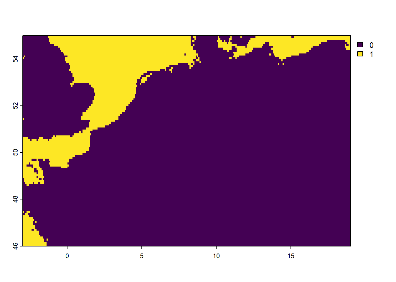
We see that the water raster is in WGS84 geographical coordinates, and with values 1 (water) and 0 (land). Thus, these two values represent classes, therefore we could also denote them with values 0 = water and 1 = land (thus reversed the values for both classes), or with any other class value (e.g. “a” and “b”).
Now, let’s project the water raster from WGS84 coordinates to ‘ETRS89-extended / LAEA Europe’ as done earlier, and we assign it to an object water_laea:
If we now inspect the resultant object, we notice something strange:
### inspect
water_laea
## class       : SpatRaster
## dimensions  : 167, 263, 1  (nrow, ncol, nlyr)
## resolution  : 6453.056, 6453.056  (x, y)
## extent      : 3318567, 5015721, 2541004, 3618665  (xmin, xmax, ymin, ymax)
## coord. ref. : ETRS89-extended / LAEA Europe
## source(s)   : memory
## name        : water
## min value   :     0
## max value   :     1
plot(water_laea)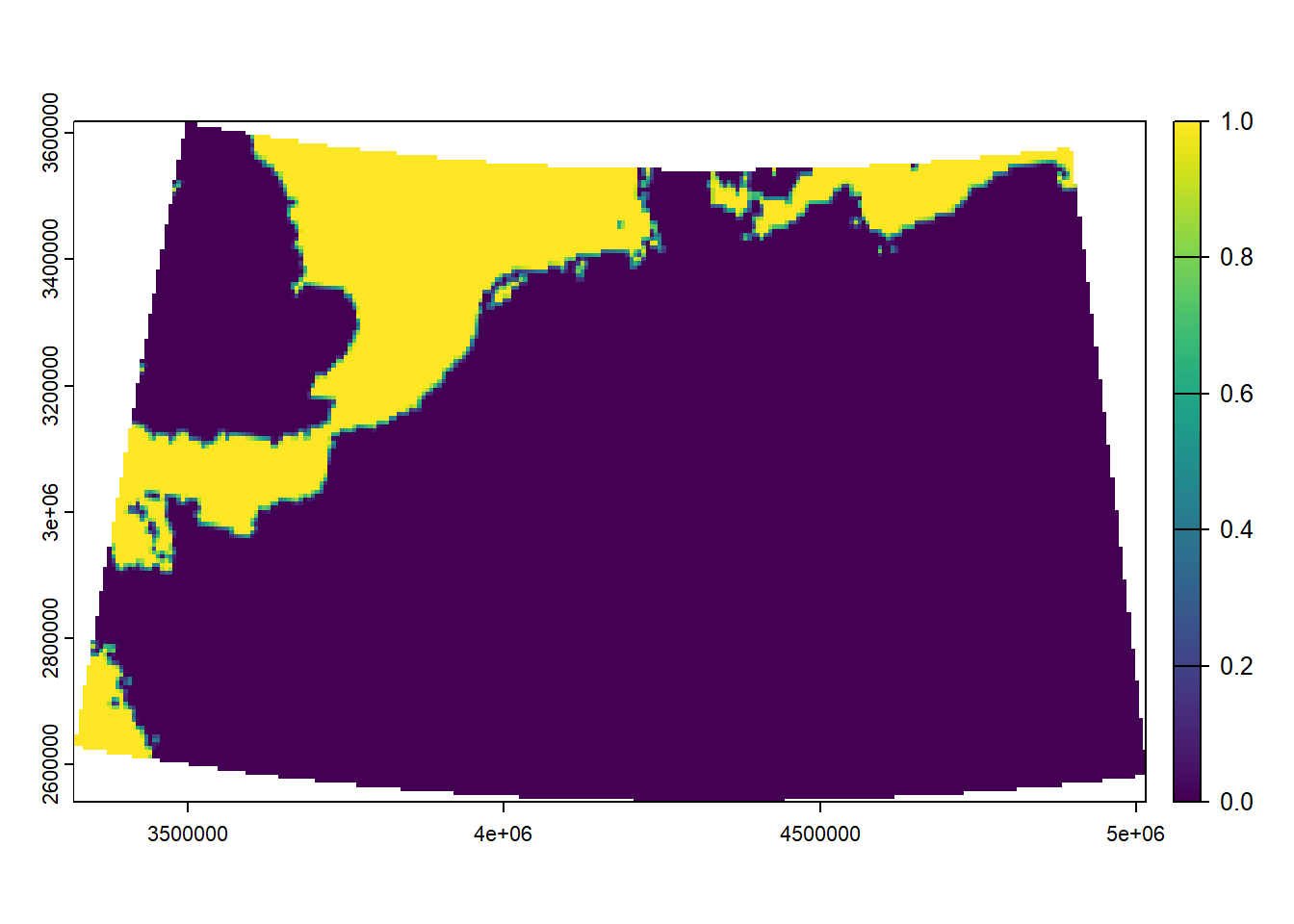
Whereas we earlier saw that the water raster only contains the values 0 and 1, after projection the water_laea raster seems to also contain values that are not exclusively 0 or 1: there are grid cells that are plotted in a different colour than just the colours for values 0 or 1.
Let’s check the values by creating a frequency table using the freq function:
But wait, it seems now that also object water_laea only contains the values 0 and 1 (and NA: those grid cells that are beyond the study area after projection!). What is going on? This does not match with the plot!
If we look at the helpfile of the freq function (run ?freq), then we see that there is an input argument digits which has the default value 0. Thus, the resultant table only shows frequencies after rounding the values to 0 digits! Let’s check the frequencies when rounding to 1 digit:
### Create frequency table (with 1 decimal rounding)
freq(water_laea, digits = 1)
##    layer value count
## 1      1   0.0 31256
## 2      1   0.1   124
## 3      1   0.2   122
## 4      1   0.3   106
## 5      1   0.4   106
## 6      1   0.5    83
## 7      1   0.6   111
## 8      1   0.7   103
## 9      1   0.8   101
## 10     1   0.9   120
## 11     1   1.0  5259
Indeed, now we see that the raster values in water_laea do not exclusively contain values 0 or 1! This is problematic, as the original data only contained 2 nominal classes, and after projecting it to a different CRS we now suddenly have a range of values even between and beyond the two values allowed…
When projecting (or resampling) raster layers, the default behaviour is bilinear interpolation: see the documentation of the ?project or ?resample functions: the default argument is method = "bilinear". Thus, when projecting or resampling a raster with class values 0 or 1, a grid cell that will be situated at the edge of water and land will be assigned a value that is interpolated between the values 0 and 1 (using bilinear interpolation: interpolation in different directions).
This explains this erroneous behaviour when working with categorical rasters!
A solution to project and/or resample categorical rasters correctly (thus by preserving the discrete class values as the only possible grid cell values), is to not do bilinear interpolation, but to do nearest neighbour assignment! Thus, using the project or resample function, we could set the argument method to value “near” for using the nearest neighbour. Let’s demonstrate:
### Project to LAEA, now using nearest neighbour assignment
water_laea <- project(water,
                      crs("+init=epsg:3035"),
                      method = "near") # nearest neighbour assignment

# Explore
water_laea
## class       : SpatRaster
## dimensions  : 167, 263, 1  (nrow, ncol, nlyr)
## resolution  : 6453.056, 6453.056  (x, y)
## extent      : 3318567, 5015721, 2541004, 3618665  (xmin, xmax, ymin, ymax)
## coord. ref. : ETRS89-extended / LAEA Europe
## source(s)   : memory
## name        : water
## min value   :     0
## max value   :     1

# Create frequency table (with 1 decimal rounding)
freq(water_laea, digits = 1)
##   layer value count
## 1     1     0 31752
## 2     1     1  5739

# Plot
plot(water_laea)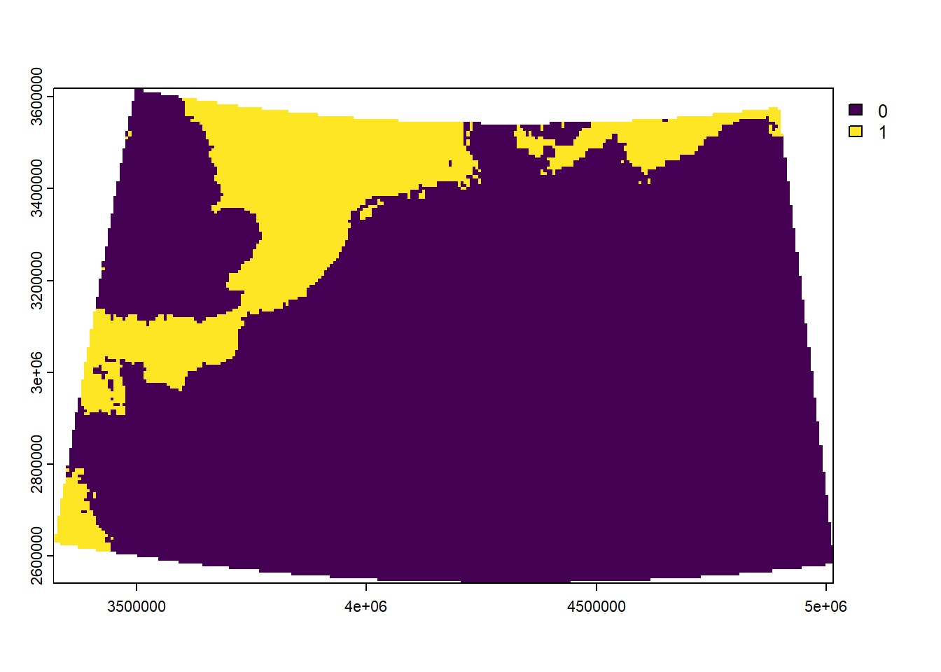
Indeed: now it seems that the projected object water_laea still only contains values 0 or 1, still coding for land and water, respectively! Let’s verify:
### Create frequency table (with 1 decimal rounding)
freq(water_laea, digits = 1)
##   layer value count
## 1     1     0 31752
## 2     1     1  5739
Thus, be extra careful when processing categorical rasters, especially when projecting or resampling!