B Loading raster data
Instead of loading WorldClim data via the getData function as used in section 3, we can download the raster data from the WorldClim website and load the raster layers from disk. First, download the file wc2.1_5m_bio.zip from the WorldClim website, and store (and unzip!) it in an appropriate place (e.g. the folder “wc2.1_5m” inside the “data/worldclim” folder). Then, we can load the data into a raster using the rast function from the terra package. As input to the rast function, we need a character vector with the names of the raster files we want to load. This character vector we can create in different ways.
The simplest, but possibly not the best way, is to use the list.files function, which list all the files in a specified directory (possibly after matching for a certain pattern):
### List all files in a specified directory
list.files("data/worldclim/wc2.1_5m")
##  [1] "wc2.1_5m_bio_1.tif"  "wc2.1_5m_bio_10.tif" "wc2.1_5m_bio_11.tif" "wc2.1_5m_bio_12.tif"
##  [5] "wc2.1_5m_bio_13.tif" "wc2.1_5m_bio_14.tif" "wc2.1_5m_bio_15.tif" "wc2.1_5m_bio_16.tif"
##  [9] "wc2.1_5m_bio_17.tif" "wc2.1_5m_bio_18.tif" "wc2.1_5m_bio_19.tif" "wc2.1_5m_bio_2.tif"
## [13] "wc2.1_5m_bio_3.tif"  "wc2.1_5m_bio_4.tif"  "wc2.1_5m_bio_5.tif"  "wc2.1_5m_bio_6.tif"
## [17] "wc2.1_5m_bio_7.tif"  "wc2.1_5m_bio_8.tif"  "wc2.1_5m_bio_9.tif"
Note that indeed 19 files (.tif files) are listed in the folder “data/worldclim/wc2.1_5m”.
However, also note the order of the files! Namely, although the first file is “wc2.1_5m_bio_1.tif”, the second file is “wc2.1_5m_bio_10.tif” and not “wc2.1_5m_bio_2.tif”! This is because the order of the files can depend on your operating system (e.g. Windows) and settings. Thus, although all files can be retrieved (and thus loaded into R) quickly, you have to be very very careful in checking their order!
A more robust way would thus be to use the paste or paste0 function (the former by default has a space as the separator [but this can be changed], whereas the latter will paste different text strings together without any separator). Thus, the vector of 19 file names in the correct order can be constructed using:
### Create a vector with names
paste0("wc2.1_5m_bio_", 1:19, ".tif")
##  [1] "wc2.1_5m_bio_1.tif"  "wc2.1_5m_bio_2.tif"  "wc2.1_5m_bio_3.tif"  "wc2.1_5m_bio_4.tif"
##  [5] "wc2.1_5m_bio_5.tif"  "wc2.1_5m_bio_6.tif"  "wc2.1_5m_bio_7.tif"  "wc2.1_5m_bio_8.tif"
##  [9] "wc2.1_5m_bio_9.tif"  "wc2.1_5m_bio_10.tif" "wc2.1_5m_bio_11.tif" "wc2.1_5m_bio_12.tif"
## [13] "wc2.1_5m_bio_13.tif" "wc2.1_5m_bio_14.tif" "wc2.1_5m_bio_15.tif" "wc2.1_5m_bio_16.tif"
## [17] "wc2.1_5m_bio_17.tif" "wc2.1_5m_bio_18.tif" "wc2.1_5m_bio_19.tif"
Now, we can use this, together with the folder name, to construct valid path names to the locations of the files, and load these files into a raster:
### Load all raster using the vector with names
bio <- rast(paste0("data/worldclim/wc2.1_5m/wc2.1_5m_bio_", 1:19, ".tif"))
Lets check the object bio that is created above:
### Explore
bio
## class       : SpatRaster
## dimensions  : 2160, 4320, 19  (nrow, ncol, nlyr)
## resolution  : 0.08333333, 0.08333333  (x, y)
## extent      : -180, 180, -90, 90  (xmin, xmax, ymin, ymax)
## coord. ref. : lon/lat WGS 84 (EPSG:4326)
## sources     : wc2.1_5m_bio_1.tif
##               wc2.1_5m_bio_2.tif
##               wc2.1_5m_bio_3.tif
##               ... and 16 more source(s)
## names       : wc2.1~bio_1, wc2.1~bio_2, wc2.1~bio_3, wc2.1~bio_4, wc2.1~bio_5, wc2.1~bio_6, ...
## min values  :   -54.73946,     1.00000,    9.063088,       0.000,     -29.700,     -72.501, ...
## max values  :    31.05112,    21.73333,  100.000000,    2373.261,      48.265,      26.300, ...
names(bio)
##  [1] "wc2.1_5m_bio_1"  "wc2.1_5m_bio_2"  "wc2.1_5m_bio_3"  "wc2.1_5m_bio_4"  "wc2.1_5m_bio_5"
##  [6] "wc2.1_5m_bio_6"  "wc2.1_5m_bio_7"  "wc2.1_5m_bio_8"  "wc2.1_5m_bio_9"  "wc2.1_5m_bio_10"
## [11] "wc2.1_5m_bio_11" "wc2.1_5m_bio_12" "wc2.1_5m_bio_13" "wc2.1_5m_bio_14" "wc2.1_5m_bio_15"
## [16] "wc2.1_5m_bio_16" "wc2.1_5m_bio_17" "wc2.1_5m_bio_18" "wc2.1_5m_bio_19"
The names of the raster layers are not very convenient, so it is better to rename them “bio1”, “bio2”, …, “bio19”. If we are certain about the order of the layers (bioclimatic variable 1, 2, …, 19 and not 1, 10, 11, … 19, 2, … 9 as was the result of the list.files function call used above), then we can use the `paste0’ function here as well:
Alternatively, especially if you are not certain about the order of the layers, you can opt for a different solution to rename the layers, using the gsub function. The gsub function finds patterns in a string and replaces it with another string. Here, we can first remove the string “wc2.1_5m_” (i.e. replacing it with an empty string: ““), and then remove the underscore between”bio” and the layer number:
### alternatively, replace parts of a name
names(bio) <- gsub(names(bio), pattern = "wc2.1_5m_", replacement = "")
names(bio) <- gsub(names(bio), pattern = "_", replacement = "")
names(bio)
##  [1] "bio1"  "bio2"  "bio3"  "bio4"  "bio5"  "bio6"  "bio7"  "bio8"  "bio9"  "bio10" "bio11" "bio12"
## [13] "bio13" "bio14" "bio15" "bio16" "bio17" "bio18" "bio19"
The raster bio as created above is now the same as the object loaded using the worldclim_global function as done in section 3!
However, if we would not be careful about the order of the layers/files, and would assign the wrong names to the raster layers, we can go completely wrong:
### loading multiple files the wrong was
wrongStack <- rast(list.files("data/worldclim/wc2.1_5m", full.names = TRUE))
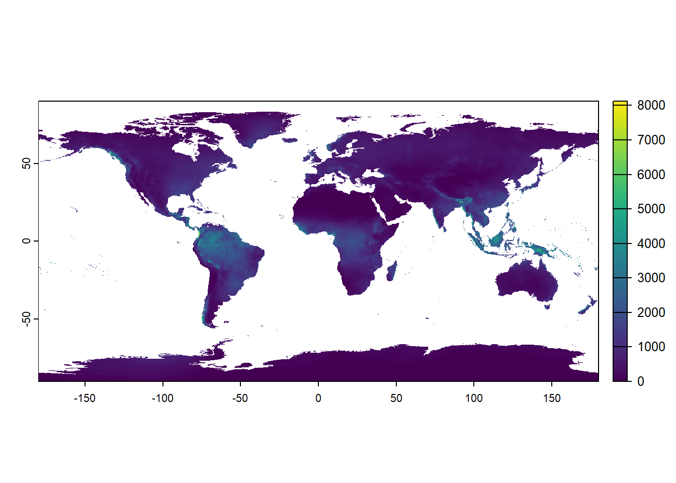
names(wrongStack) <- paste0("bio", 1:19)Namely, plotting the global pattern of annual rainfall (bio12) now suggests that many of the known desert and arid areas (e.g. the Sahel and Sahara) are actually among the wettest parts of the Earth:
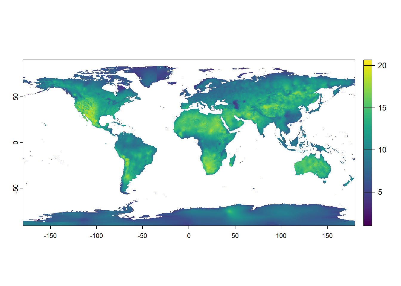
However, this is simply because we’ve assigned the wrong names to the raster layers: actually “bio12” is now the 4th layer in the raster (it is the 4th element in the list.files function call and thus the 4th layer that is loaded into the stack). Plotting the 4th layer of the stack wrongStack now actually gives sensible results, as now the tropical rainforest areas the wettest parts on Earth: