Chapter 3 Raster data
Raster data can also be loaded from either a local file, or from online sources. Like in the previous section, data can be loaded from online sources using the geodata package. To load raster data from a local file, we could use terra’s rast function, which loads raster data into an object of class SpatRaster.
3.1 Loading data from online sources
We will use long term bio-climatic data from WorldClim. We can either download the data from the WorldClim website and then load it into R, or use the geodata package; using one of the worldclim_global, worldclim_country or worldclim_tile functions (respectively to load WorldClim data with a global extent, or for a specific country or set of countries, or for a specified longitude-latitude extent).
Here, we will focus on the Historical climate data at 5 arc-minutes spatial resolution (but we could also focus on data at 10, 2.5, 0.5 minutes resolution, the latter one thus being 30 seconds), where we focus on the Bioclimatic variables. We will load the data at 5 arc-minutes spatial resolution using the worldclim_global function directly from R (note that downloading might take some time, especially at higher resolutions), in which case global data will be downloaded (but see Appendix B for other ways of loading raster data into R):
### Download global worldclim data at 5 minute resolution
bio <- worldclim_global(var = "bio", # "tmin", "tmax", "tavg", "prec", "wind", "vapr", or "bio"
                        res = 5, # resolution: 10, 5, 2.5, or 0.5 (minutes of a degree)
                        path = "data/worldclim")
When the data has succesfully been downloaded, running this code again will not download the files again, but rather simply load the downloaded files instead of downloading the files again.
Like done above with the cities object, we can first explore the bio object:
# general overview
bio
## class       : SpatRaster
## dimensions  : 2160, 4320, 19  (nrow, ncol, nlyr)
## resolution  : 0.08333333, 0.08333333  (x, y)
## extent      : -180, 180, -90, 90  (xmin, xmax, ymin, ymax)
## coord. ref. : lon/lat WGS 84 (EPSG:4326)
## sources     : wc2.1_5m_bio_1.tif
##               wc2.1_5m_bio_2.tif
##               wc2.1_5m_bio_3.tif
##               ... and 16 more source(s)
## names       : wc2.1~bio_1, wc2.1~bio_2, wc2.1~bio_3, wc2.1~bio_4, wc2.1~bio_5, wc2.1~bio_6, ...
## min values  :   -54.73946,     1.00000,    9.063088,       0.000,     -29.700,     -72.501, ...
## max values  :    31.05112,    21.73333,  100.000000,    2373.261,      48.265,      26.300, ...
# information on the coordinate system
crs(bio, proj = TRUE, describe = TRUE)
## name authority code area extent proj
## 1 WGS 84 EPSG 4326 World -180, 180, -90, 90 +proj=longlat +datum=WGS84 +no_defs# names of the different raster layers
names(bio)
## [1] "wc2.1_5m_bio_1" "wc2.1_5m_bio_2" "wc2.1_5m_bio_3" "wc2.1_5m_bio_4" "wc2.1_5m_bio_5"
## [6] "wc2.1_5m_bio_6" "wc2.1_5m_bio_7" "wc2.1_5m_bio_8" "wc2.1_5m_bio_9" "wc2.1_5m_bio_10"
## [11] "wc2.1_5m_bio_11" "wc2.1_5m_bio_12" "wc2.1_5m_bio_13" "wc2.1_5m_bio_14" "wc2.1_5m_bio_15"
## [16] "wc2.1_5m_bio_16" "wc2.1_5m_bio_17" "wc2.1_5m_bio_18" "wc2.1_5m_bio_19"We see that the names of the raster layers are quite long, as they include the identifier of the WorldClim dataset used (version 2.1) as well as the resolution (5 minutes). We can simplify the names of the layers by simply giving them the names “bio1”, “bio2”, …, “bio19”, for which we can use the paste0 function to concatenate strings:
names(bio) <- paste0("bio",1:19)
names(bio)
##  [1] "bio1"  "bio2"  "bio3"  "bio4"  "bio5"  "bio6"  "bio7"  "bio8"  "bio9"  "bio10" "bio11" "bio12"
## [13] "bio13" "bio14" "bio15" "bio16" "bio17" "bio18" "bio19"As we see above, the object bio is a SpatRaster with 19 layers with names “bio1”, “bio2”, …, “bio19”, with global-scale data.
According to the WorldClim website, these bioclimatic variables contain the following information:
| layer | Bioclimatic variable |
|---|---|
| bio1 | Annual Mean Temperature |
| bio2 | Mean Diurnal Range (Mean of monthly max temp - min temp) |
| bio3 | Isothermality (BIO2 / BIO7 * 100) |
| bio4 | Temperature Seasonality (standard deviation * 100) |
| bio5 | Max Temperature of Warmest Month |
| bio6 | Min Temperature of Coldest Month |
| bio7 | Temperature Annual Range (BIO5-BIO6) |
| bio8 | Mean Temperature of Wettest Quarter |
| bio9 | Mean Temperature of Driest Quarter |
| bio10 | Mean Temperature of Warmest Quarter |
| bio11 | Mean Temperature of Coldest Quarter |
| bio12 | Annual Precipitation |
| bio13 | Precipitation of Wettest Month |
| bio14 | Precipitation of Driest Month |
| bio15 | Precipitation Seasonality (Coefficient of Variation) |
| bio16 | Precipitation of Wettest Quarter |
| bio17 | Precipitation of Driest Quarter |
| bio18 | Precipitation of Warmest Quarter |
| bio19 | Precipitation of Coldest Quarter |
Next to these bioclimatic variables, the function can also be used to download other WorldClim variables, inclusing monthly climate data for minimum, mean, and maximum temperature, precipitation, solar radiation, wind speed, water vapor pressure, and for total precipitation.
The geodata package includes also other functions to download other datasets (see function documentation for data source and more information):
cropland: cropland distribution data;elevation_3s,elevation_30sorelevation_global: elevation data, derived from the hole-filed SRTM digital elevation model;footprint: the human “footprint” estimate of the direct and indirect human pressures on the environment;landcover: landcover data for (most of) the world;population: population density data;soil_world: global soil data (for Africa see also functionsoil_afas well as related functions);sp_occurrence: species occurrence data from the Global Biodiversity Information Facility (GBIF).
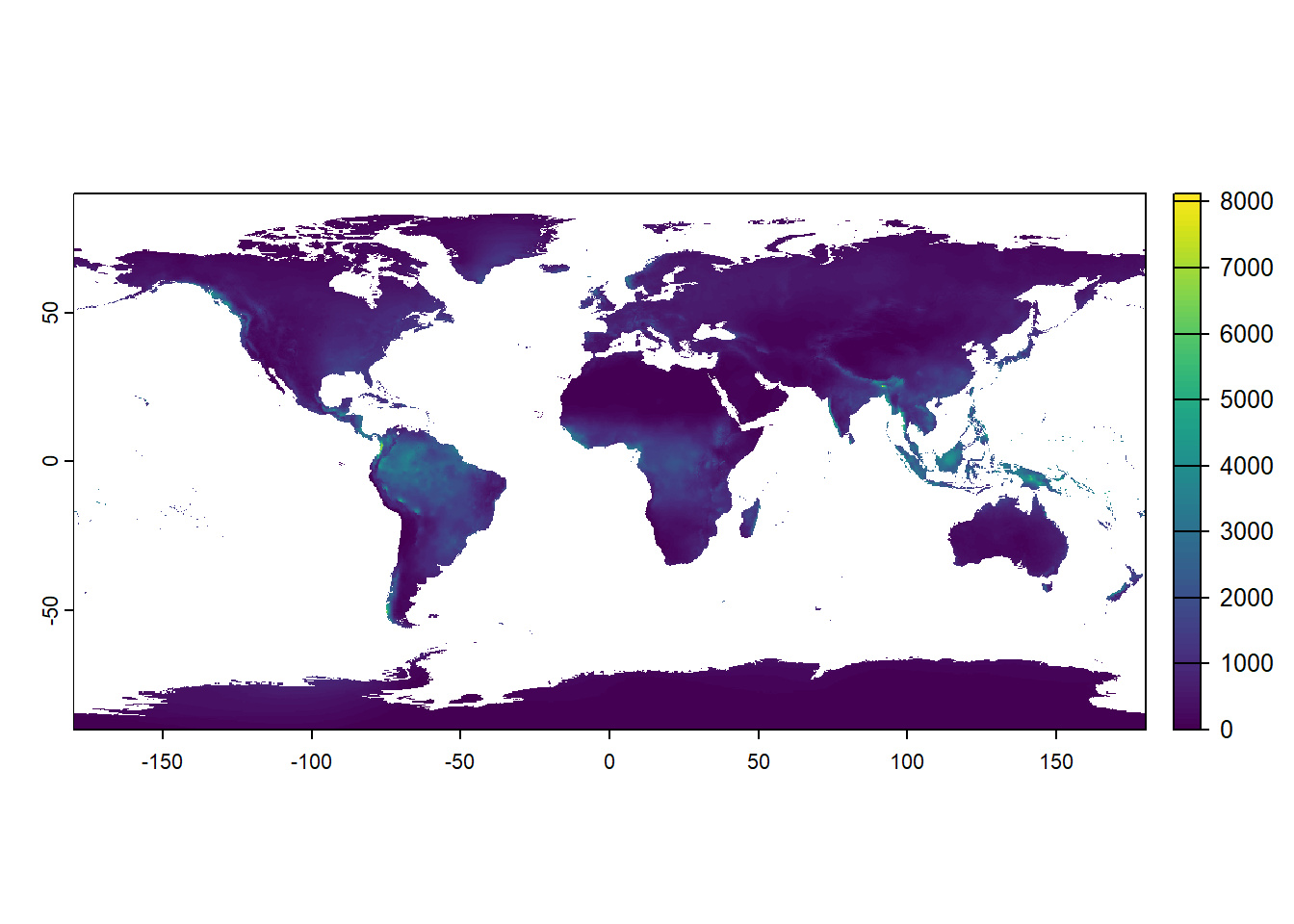
We can plot the global pattern of annual precipitation (bio12) by just retrieving the 12th element of the object bio (or the object with name “bio12”) and plot that:
3.2 Loading data from local files
Suppose that we have 2 local raster files that we also want to load into R. First download water.tif and mask.tif, and store them in an appropriate folder (e.g. in a “data” folder). Then, we can load them into R using the rast function, and inspect the result by printing it to the console:
### Load local rasters into R
water <- rast("data/water.tif")
mask <- rast("data/mask.tif")

# inspect
water
## class       : SpatRaster
## dimensions  : 108, 264, 1  (nrow, ncol, nlyr)
## resolution  : 0.08333333, 0.08333333  (x, y)
## extent      : -3, 19, 46, 55  (xmin, xmax, ymin, ymax)
## coord. ref. : lon/lat WGS 84 (EPSG:4326)
## source      : water.tif
## name        : water
## min value   :     0
## max value   :     1
mask
## class       : SpatRaster
## dimensions  : 108, 264, 1  (nrow, ncol, nlyr)
## resolution  : 0.08333333, 0.08333333  (x, y)
## extent      : -3, 19, 46, 55  (xmin, xmax, ymin, ymax)
## coord. ref. : lon/lat WGS 84 (EPSG:4326)
## source      : mask.tif
## name        : mask
## min value   :    1
## max value   :    1
We see in the output printed above that both layers are loaded with identical extent and resolution, both in WGS84 geographical coordinates.
Now, let’s inspect both layers by plotting them and creating a frequency table of raster grid cell values using the freq function:
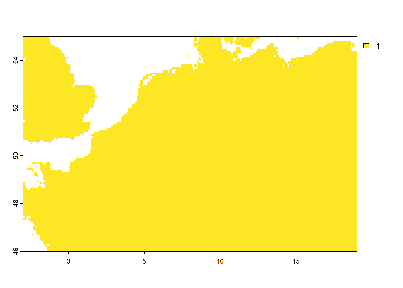
As we can see, the mask layer has the value 1 for the terrestrial part of the study area, and value NA elsewhere.
### inspect the water layer
freq(water)
##   layer value count
## 1     1     0 23926
## 2     1     1  4586
plot(water)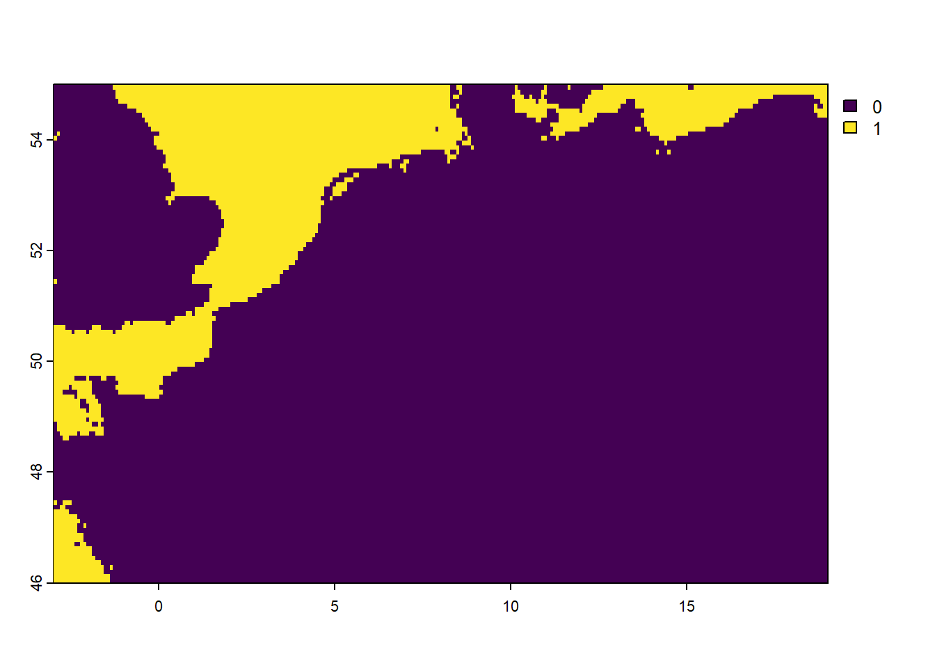
As we can see, the water layer contains only the values 0 or 1, with 1 representing water (sea or ocean), and value 0 representing land.