Chapter 4 Processing raster data
4.1 Cropping rasters
As we saw earlier, the different raster objects that we have loaded (bio, water, and mask) have different extents:
ext(bio)
## SpatExtent : -180, 180, -90, 90 (xmin, xmax, ymin, ymax)
ext(water)
## SpatExtent : -3, 19, 46, 55 (xmin, xmax, ymin, ymax)
ext(mask)
## SpatExtent : -3, 19, 46, 55 (xmin, xmax, ymin, ymax)
Namely, the bio raster has a global extent, whereas the other two layers have a west European extent.
In order to focus our analyses to the area of interest, we can crop the object bio from a global extent to a smaller extent using the crop function, while supplying it with an extent to crop the raster to (here the output of the ext(mask) function):
Alternatively, we could also crop rasters manually if we know the coordinates to which we want to crop the raster: the extent function can also take as argument a vector of values in the order of: xmin, xmax, ymin, ymax. Thus, we could also crop the bio raster to longitude ranging from -3 to 19 degrees, and latitude ranging from 46 to 55 degrees:
Let’s check whether bio now has a smaller extent:
ext(bio)
## SpatExtent : -3, 19, 46, 55 (xmin, xmax, ymin, ymax)
plot(bio[[12]])
points(cities, pch=16, col="black")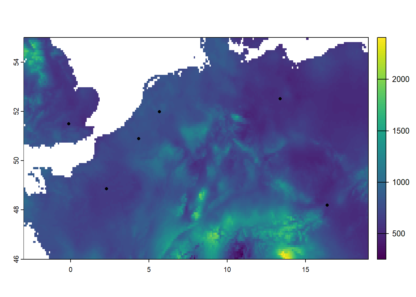
As we can see, the bio raster now has a much smaller extent!
4.2 Subsetting layers
Instead of focussing on all 19 bioclimatic variables, let’s focus on 4 variables: Annual Mean Temperature (bio1), Temperature Seasonality (bio4), Max Temperature of Warmest Month (bio5) and Annual Precipitation (bio12). We can use the subset function to subset layers from a raster. Let’s assign the subsetted raster to an object called bio_sub:
Let’s check the number of layers in bio_sub, their names, and plot it:
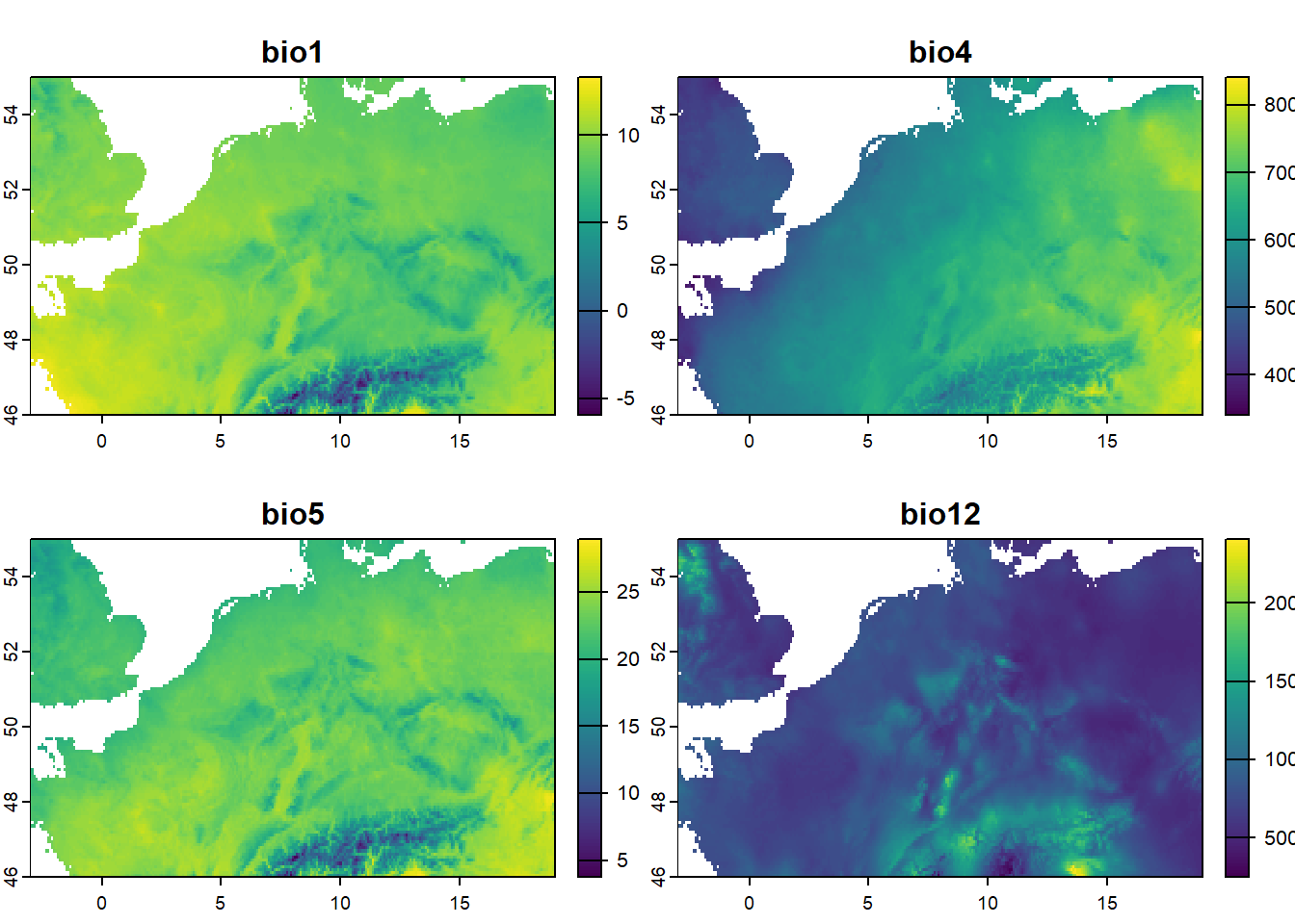
As we can see, the plot function will automatically plot all (here: 4) layers in the raster.
4.3 Calculating with rasters
We can easily see a quick summary of the values in each layer in the raster object using the summary function:
summary(bio_sub)
##       bio1             bio4            bio5            bio12
##  Min.   :-5.922   Min.   :341.4   Min.   : 3.789   Min.   : 253.0
##  1st Qu.: 8.183   1st Qu.:563.2   1st Qu.:21.458   1st Qu.: 624.0
##  Median : 8.965   Median :630.8   Median :22.749   Median : 741.0
##  Mean   : 8.791   Mean   :623.8   Mean   :22.455   Mean   : 785.8
##  3rd Qu.: 9.951   3rd Qu.:697.8   3rd Qu.:23.768   3rd Qu.: 850.0
##  Max.   :13.288   Max.   :840.9   Max.   :28.928   Max.   :2406.0
##  NA's   :4586     NA's   :4586    NA's   :4586     NA's   :4586
To retrieve global statistics (i.e. statistics that summarize values of an entire raster), we can use the global function. For example, to compute the maximum value of the raster layers in bio_sub:
global(bio_sub, fun = "max", na.rm = TRUE)
##             max
## bio1    13.2875
## bio4   840.9453
## bio5    28.9280
## bio12 2406.0000
Here we use na.rm = TRUE to remove missing values (NA) before computing the maximum.
We can apply basic mathematical operiations (multiplication, addition etc) directly on raster objects. For example, the BIO3 variable (Isothermality) is computed as BIO2 / BIO7 * 100. Thus, we could compute it ourselves and verify by comparing the result with bio3:
We see that the range in values is equal (we could also plot them to verify that they are identical).
4.4 Working with classes
We saw earlier that the values of the water object are only 1 (denoting water) or 0 (denoting land). Suppose that we want to know for each city in cities how far it is from the sea or ocean, we may want to create a distance to water raster. A handy way of getting such raster is by first creating a raster that the value 1 for grid cells that are water, and value NA elsewhere. Let’s create such a layer and call it dwater:
### Get raster with 1 = water and NA else
dwater <- water            # first we copy the water raster
names(dwater) <- "dwater"  # assign it a more meaningful name
dwater[dwater == 0] <- NA  # replace the value 0 with the value NA

# check by plotting and creating a frequency table
freq(dwater)
##   layer value count
## 1     1     1  4586
plot(dwater)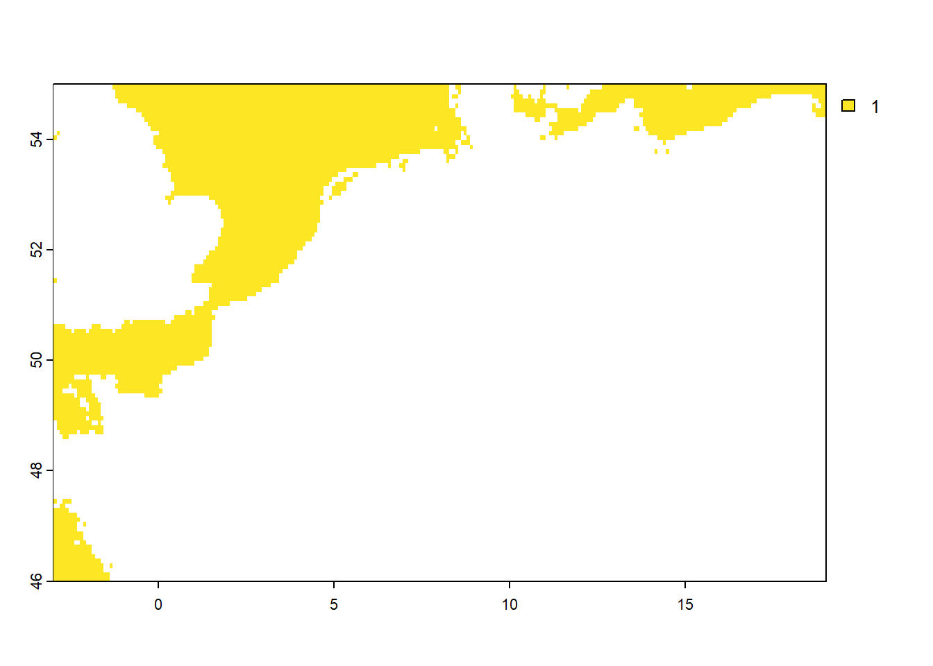
4.5 Computing distances
Given that we have created the dwater raster above, with values 1 (water) and NA (elsewhere), we can now conveniently compute the distance to water using the distance function from the terra package. This function computes, for each grid cell, the Euclidean distance (thus ‘as the crow flies’) to the nearest grid cell that is not NA (thus, as per the creation of dwater: those grid cells that are water!):
### Compute distance to water
dwater <- distance(dwater) # note that this may take several seconds to compute
## |---------|---------|---------|---------|=========================================
names(dwater) <- "dwater"  # assign it a more meaningful name
dwater <- dwater / 1000    # since the distance is returned in meters, convert km
plot(dwater)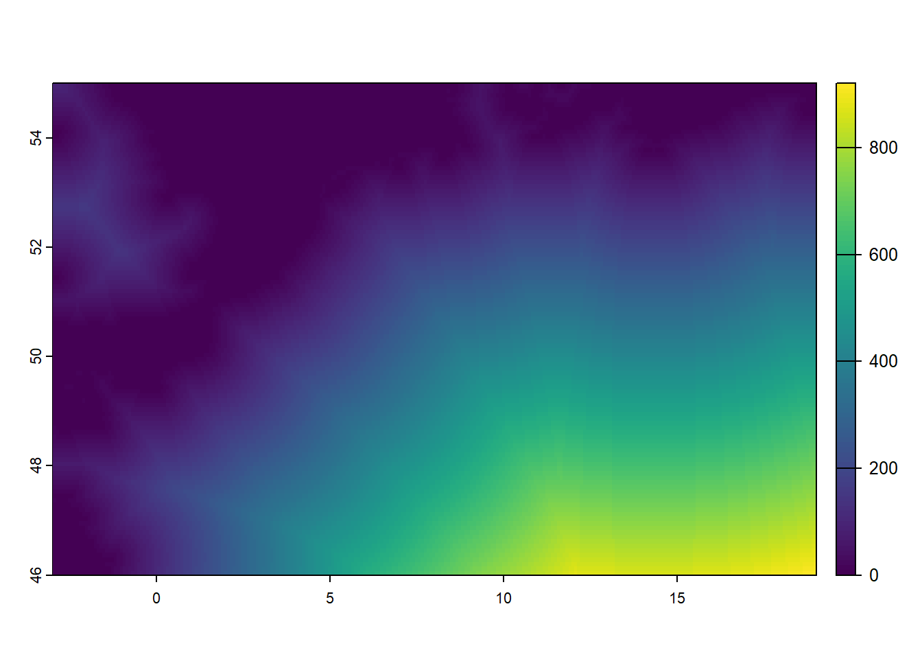
4.6 Merging raster layers
We now have multiple objects with raster data: bio (with all 19 bioclimatic variables), bio_sub (with our 4 selected layers), water, dwater, as well as a raster with masking information: mask.
We can combine different layers into a single raster (assuming that these objects are in the same CRS, extent and resolution) using the c function. Let’s merge bio_sub and dwater into a single raster object called rstack:
### Combine the different raster objects into a single raster
rstack <- c(bio_sub, dwater)

# inspect
rstack
## class       : SpatRaster
## dimensions  : 108, 264, 5  (nrow, ncol, nlyr)
## resolution  : 0.08333333, 0.08333333  (x, y)
## extent      : -3, 19, 46, 55  (xmin, xmax, ymin, ymax)
## coord. ref. : lon/lat WGS 84 (EPSG:4326)
## source(s)   : memory
## names       :      bio1,     bio4,   bio5, bio12,   dwater
## min values  : -5.921834, 341.4172,  3.789,   253,   0.0000
## max values  : 13.287500, 840.9453, 28.928,  2406, 920.5839
names(rstack)
## [1] "bio1"   "bio4"   "bio5"   "bio12"  "dwater"
4.7 Masking rasters
Now that we have combined all rasters with environmental data into a single object rstack, we can mask the object using the mask: this creates a new raster object that has the same values as the input object, except for the cells that are NA in a ‘mask’ object:
### Mask the values in the rstack object using the mask layer
rstack <- mask(rstack, mask)

# Check by plotting
plot(rstack)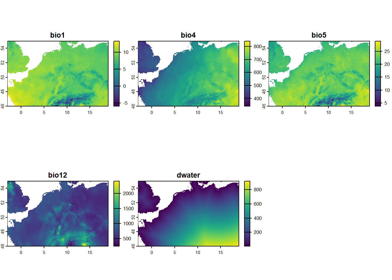
We now have a single raster object rstack with 5 layers: 4 selected bioclimatic variables (with adjusted values), and a layer with the distance to the sea or ocean (in km). All values in the resulting raster are masked using the mask grid, so that grid cells that contain water are masked to value NA.
4.8 Resampling rasters
Especially when working with many different raster objects, it often happens that the raster objects do not match (in terms of origin, extent and resolution), even when they are in the same CRS (see section 5 for [re]-projecting) raster layers into a different CRS). In such cases, it could help to crop or extend a/the raster (using the crop or extend functions), or to (dis)aggregate rasters (using the aggregate or disagg functions; where aggregate lowers the resolution by a specified factor and with specified function, whereas disagg creates a raster with a higher resolution - thus smaller grid cells - than the original raster by a specified factor using a specified function).
Also, it may be needed to resample rasters, using the resample function, which transfers values between non matching raster objects (in terms of origin and resolution) and uses bilinear interpolation or nearest neighbour assignment to assign values to resampled grid cells.
Note that aggregating, disaggregating and resampling rasters with categorical values (classes) should only be done with great care: see Appendix C.
4.9 Other processing methods
For more information on processing spatial data, see Appendix D. For a list with the most important methods of processing spatial data using the terra package, grouped by theme, see: