Spatial Data and Analyses in R

Chapter 2 Vector data

2.1 Loading data from local files

Let’s load the locations of these cities into R: download the file cities.zip into your “data” folder, and unzip it to the “cities” subfolder, so that the folder “data/cities” contains the 4 unzipped files that together make a shapefile. Then, we can use the vect function from the terra package to load the shapefile into R (see Appendix A for other ways of loading vector data into R):

### Load the cities shapefile into a vector layer
cities <- vect("data/cities/cities.shp")

Now, we can explore the properties of the cities object using e.g.:

# overall overview
cities
##  class       : SpatVector 
##  geometry    : points 
##  dimensions  : 6, 1  (geometries, attributes)
##  extent      : -0.1249526, 16.38053, 48.19038, 52.5132  (xmin, xmax, ymin, ymax)
##  source      : cities.shp
##  coord. ref. : lon/lat WGS 84 (EPSG:4326) 
##  names       :       city
##  type        :      <chr>
##  values      : Wageningen
##                     Paris
##                    London

# class
class(cities)
## [1] "SpatVector"
## attr(,"package")
## [1] "terra"

# spatial extent/bounding box
ext(cities)
## SpatExtent : -0.124952562617393, 16.3805349488525, 48.1903797097879, 52.5132034875388 (xmin, xmax, ymin, ymax)

# retrieve information on coordinate system
crs(cities, proj = TRUE) # crs in PROJ-string notation
## [1] "+proj=longlat +datum=WGS84 +no_defs"
crs(cities, describe = TRUE) # EPSG code and other info
##     name authority code area         extent
## 1 WGS 84      EPSG 4326 <NA> NA, NA, NA, NA
crs(cities, proj = TRUE, describe = TRUE) # combined
##     name authority code area         extent                                proj
## 1 WGS 84      EPSG 4326 <NA> NA, NA, NA, NA +proj=longlat +datum=WGS84 +no_defs

# columns with properties per location
names(cities)
## [1] "city"

# header of all properties
head(cities)
##         city
## 1 Wageningen
## 2      Paris
## 3     London
## 4     Berlin
## 5   Brussels
## 6     Vienna

# retrieve inforamtion on geometry (e.g. coordinates)
geom(cities)
##      geom part          x        y hole
## [1,]    1    1  5.6634428 51.98553    0
## [2,]    2    1  2.2917644 48.85816    0
## [3,]    3    1 -0.1249526 51.49865    0
## [4,]    4    1 13.3766394 52.51320    0
## [5,]    5    1  4.3420292 50.89498    0
## [6,]    6    1 16.3805349 48.19038    0

Above, we can see that the loaded shapefile has coordinates that are stored in the ‘WGS84’ geographical coordinate system (EPSG: 4326).

We can use a dynamic mapping library like LeafletJS (see Leaflet for R) to plot geographical data in an interactive map. We can map the locations stored in cities as basic markers on a Leaflet map, with a popup that shows the city name, using a very simple syntax:

### Plot on a dynamic leaflet map
plet(cities)

2.2 Loading data from online sources

We can use the gadm function from the geodata package to (down)load the outline of administrative boundaries for any country in the world; they are read in as a SpatVector polygon object. As input it needs ISO3 country code data (see function country_codes), e.g. “NLD” for the Netherlands.

Suppose that we want to load the outline of 13 European countries that are in the vicinity of our selected cities, we could use:

### ISO3 codes for selected European countries
euroISO3 <- c("AUT", "BEL", "CHE", "CZE", "DEU", "DNK", "FRA",
              "GBR", "HUN", "ITA", "LUX", "NLD", "POL")

### Download country outline data
countries <- gadm(country = euroISO3, # vector with ISO3 names of the countries
                  level = 0, # 0: country, 1: first level of subdivision
                  path = "data/countries/") # folder where to save data
                                            # to save in temporary folder use: 
                                            # path = tempdir()

Let’s see what we now have loaded:

# explore
countries
##  class       : SpatVector 
##  geometry    : polygons 
##  dimensions  : 13, 2  (geometries, attributes)
##  extent      : -8.649996, 24.14578, 35.49292, 60.84548  (xmin, xmax, ymin, ymax)
##  source      : countries.shp
##  coord. ref. : lon/lat WGS 84 (EPSG:4326) 
##  names       : GID_0     COUNTRY
##  type        : <chr>       <chr>
##  values      :   AUT     Austria
##                  BEL     Belgium
##                  CHE Switzerland

We can see that the countries object contains 13 geometries (the 13 selected countries) and 2 attributes (the attributes “GID_0” and “COUNTRY”).

If we check the folder “data/countries”, we see that a folder “gadm” is added, with 13 files; one for each country. We could save the countries object as a shapefile, so that we can lateron load it efficiently and do not have to either download the data again, or load the 13 separately saved files. For this, we could use the writeVector function:

writeVector(countries,
            filename = "data/countries/countries.shp",
            filetype = "ESRI Shapefile")

After saving this file, we could easily load it using:

countries <- vect("data/countries/countries.shp")

Note that if we want to subset the countries object further for a specific set of countries, we could use the subset function. For example, suppose that we want to retrieve the subset with only the Netherlands and Belgium, we could use:

subset(countries, countries$GID_0 %in% c("NLD","BEL"))

In order to do this efficiently, we can specify a vector with countries to keep using the c() function, and use the %in% logical operator to keep all of those features in the countries object that has a value for the “GID_0” column that is present in the specified vector.

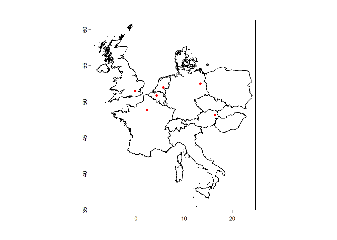
We can check the object countries by plotting it and adding the cities as (red) points:

plot(countries)
points(cities, col = "red", pch = 16) #