Spatial Data and Analyses in R

Chapter 5 Projecting data

We now have prepared 3 objects for further use: cities and countries that contain vector data (points and polygons, respectively), as well as rstack that contains a stack of raster layers.

Because these objects are in WGS84 geographical coordinates, let’s project these objects into a projection system that is convenient for western Europe: ‘ETRS89-extended / LAEA Europe’ coordinate system (EPSG: 3035). For this we can use the project function:

### Project from WGS84 to LAEA Europe
cities <- project(cities, crs("+init=epsg:3035"))
countries <- project(countries, crs("+init=epsg:3035"))
rstack <- project(rstack, crs("+init=epsg:3035"))

Let’s check the data by plotting the mean annual precipitation and overlaying the locations of the cities on them:

### Check by plotting, e.g. layer bio1
plot(rstack[["bio1"]])
points(cities, pch=16, col="black")
lines(countries)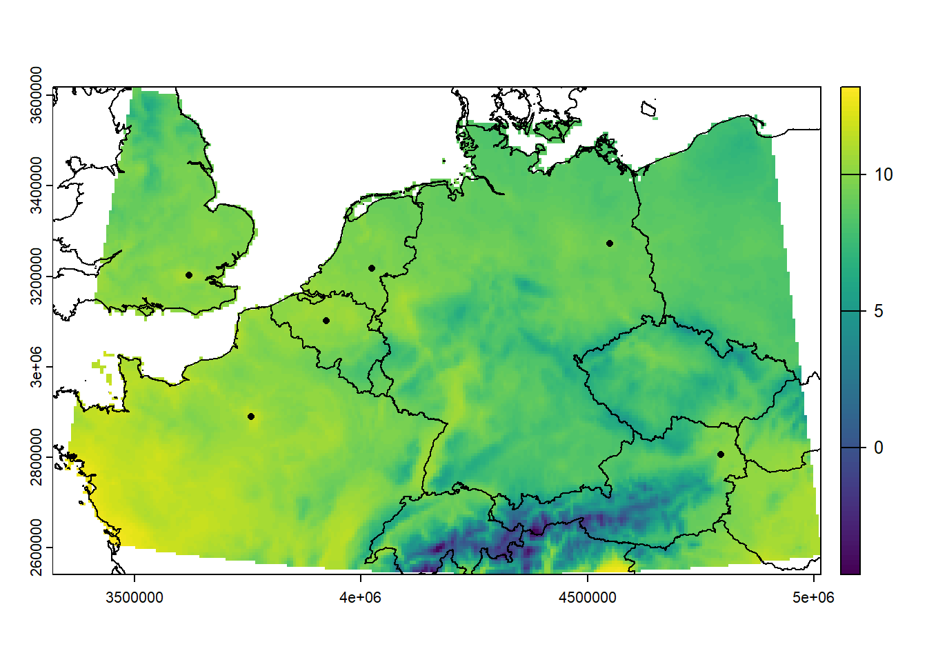

Note that (re)projecting rasters with categorical values (classes) should only be done with great care: see Appendix C.