Introduction

In these exercises, you will explore and analyse data on ecological traits of amphibians that were compiled from the literature. Traits on the size and body mass of species are included, as well as their habitat, their diel and seasonal activity patterns, and information on reproductive output. The data consists of six data files:

data_habitat.csv
data_diet.csv
data_diel.csv
data_seasonality.csv
data_breeding.csv
data_other.csv

Loading and preparing data

Create a new script file in RStudio. Download the data from Brightspace (Skills > datasets > amphibians), and store the .csv files in an appropriate folder. Load the tidyverse package and all the datasets: give the object clear and meaning names (“habitat_dat”, “diet_dat”, etc).

Before being able to work with the data, some data wrangling needs to be done:

First, transform the “habitat”, “diet”, “diel”, “seasonality”, and “breeding” dataset into longer tidy datasets. Do so by combining (for each of the five datasets) the different dummy variables (i.e., all columns in the datasets except the “Species” column) into two columns: a column with an intuitive names like “habitat”, “diet”, “diel”, “seasonality”, and “breeding”, and a column called “count” that holds the value of the dummy variable. Since this “count” column will only contain values 0, 1 and NA, filter each of the 5 tables to exclude rows where the “count” column has a NA value, and after that remove the “count” column.
In the “seasonality” dataset, separate the column “seasonality” into columns named “drywet” and “coldwarm”, based on underscore as separator.
The column “Species” is the key variable in this dataset. Check in “data_other” whether all species occur once, or whether there are multiple records per species. If there are species with more than one record, then you should remove all rows from this species from the tibble.
Finally, combine all datasets together in a tibble called dat, while keeping all species that are in “data_other” (after removing species with more than one record in the dataset). Join the datasets to “data_other” in the order as they are listed above, and use the “Species” column as the shared key column.

# Load libraries
library(tidyverse)

# Load datasets
habitat_dat <- read_csv("data/raw/amphibians/data_habitat.csv")
diet_dat <- read_csv("data/raw/amphibians/data_diet.csv")
diel_dat <- read_csv("data/raw/amphibians/data_diel.csv")
seasonality_dat <- read_csv("data/raw/amphibians/data_seasonality.csv")
breeding_dat <- read_csv("data/raw/amphibians/data_breeding.csv")
other_dat <- read_csv("data/raw/amphibians/data_other.csv")

# Made datasets tidy: pivot longer
habitat_dat <- habitat_dat %>%
  pivot_longer(!Species, names_to = "habitat", values_to = "count") %>%
  drop_na(count) %>%
  select(-count)

diet_dat <- diet_dat %>%
  pivot_longer(!Species, names_to = "diet", values_to = "count") %>%
  drop_na(count) %>%
  select(-count)

diel_dat <- diel_dat %>%
  pivot_longer(!Species, names_to = "diel", values_to = "count") %>%
  drop_na(count) %>%
  select(-count)

seasonality_dat <- seasonality_dat %>%
  pivot_longer(!Species, names_to = "seasonality", values_to = "count") %>%
  drop_na(count) %>%
  select(-count)

breeding_dat <- breeding_dat %>%
  pivot_longer(!Species, names_to = "breeding", values_to = "count") %>%
  drop_na(count) %>%
  select(-count)

# Separate "seasonality" into columns named "drywet" and "coldwarm", based on underscore as separator
seasonality_dat = seasonality_dat %>%
  separate(seasonality, into = c("drywet","coldwarm"), sep="_", remove=FALSE)

# Check whether other_dat has duplicates for Species
other_dat %>%
  group_by(Species) %>%
  mutate(count = n()) %>%
  filter(count > 1)

## # A tibble: 0 × 17
## # Groups:   Species [0]
## # ℹ 17 variables: Order <chr>, Family <chr>, Genus <chr>, Species <chr>, Body_mass_g <dbl>, Age_at_maturity_min_y <dbl>,
## #   Age_at_maturity_max_y <dbl>, Body_size_mm <dbl>, Size_at_maturity_min_mm <dbl>, Size_at_maturity_max_mm <dbl>, Longevity_max_y <dbl>,
## #   Litter_size_min_n <dbl>, Litter_size_max_n <dbl>, Reproductive_output_y <dbl>, Offspring_size_min_mm <dbl>,
## #   Offspring_size_max_mm <dbl>, count <int>

# no: 0 rows

# join by species
dat <- other_dat %>%
  left_join(habitat_dat, by = "Species") %>%
  left_join(diet_dat, by = "Species") %>%
  left_join(diel_dat, by = "Species") %>%
  left_join(seasonality_dat, by = "Species") %>%
  left_join(breeding_dat, by = "Species")
dat

## # A tibble: 41,745 × 23
##    Order Family        Genus      Species        Body_mass_g Age_at_maturity_min_y Age_at_maturity_max_y Body_size_mm Size_at_maturity_min…¹
##    <chr> <chr>         <chr>      <chr>                <dbl>                 <dbl>                 <dbl>        <dbl>                  <dbl>
##  1 Anura Allophrynidae Allophryne Allophryne ru…          31                    NA                    NA           31                     NA
##  2 Anura Allophrynidae Allophryne Allophryne ru…          31                    NA                    NA           31                     NA
##  3 Anura Allophrynidae Allophryne Allophryne ru…          31                    NA                    NA           31                     NA
##  4 Anura Allophrynidae Allophryne Allophryne ru…          31                    NA                    NA           31                     NA
##  5 Anura Allophrynidae Allophryne Allophryne ru…          31                    NA                    NA           31                     NA
##  6 Anura Allophrynidae Allophryne Allophryne ru…          31                    NA                    NA           31                     NA
##  7 Anura Allophrynidae Allophryne Allophryne ru…          31                    NA                    NA           31                     NA
##  8 Anura Allophrynidae Allophryne Allophryne ru…          31                    NA                    NA           31                     NA
##  9 Anura Allophrynidae Allophryne Allophryne ru…          31                    NA                    NA           31                     NA
## 10 Anura Allophrynidae Allophryne Allophryne ru…          31                    NA                    NA           31                     NA
## # ℹ 41,735 more rows
## # ℹ abbreviated name: ¹Size_at_maturity_min_mm
## # ℹ 14 more variables: Size_at_maturity_max_mm <dbl>, Longevity_max_y <dbl>, Litter_size_min_n <dbl>, Litter_size_max_n <dbl>,
## #   Reproductive_output_y <dbl>, Offspring_size_min_mm <dbl>, Offspring_size_max_mm <dbl>, habitat <chr>, diet <chr>, diel <chr>,
## #   seasonality <chr>, drywet <chr>, coldwarm <chr>, breeding <chr>

If you did not manage to generate the dat tibble above, then use the “Amphibian_data.csv” file and load it into a tibble called dat to be able to do the following exercises.

Some exploration of the data

First, we are going to do some exploration of the dataset dat:

Compute the number of records per order (column “Order”);
Compute the number of species for each order;
Compute mean body size (column “Body_mass_g”) and reproductive output (column “Reproductive_output_y”) per order while removing NAs in the computation of the averages. Give meaningful names tot the computed averages. Sort the resultant table such that the order with the largest average body size is in the top-row and that with the smallest body size in the bottom-row.

# Count number of records per order
dat %>%
  count(Order)

## # A tibble: 3 × 2
##   Order           n
##   <chr>       <int>
## 1 Anura       36771
## 2 Caudata      4010
## 3 Gymnophiona   964

# or use group_by() & summarize(), or use table()

# Count number of species per order
dat %>%
  count(Order, Species) %>%
  count(Order)

## # A tibble: 3 × 2
##   Order           n
##   <chr>       <int>
## 1 Anura        5971
## 2 Caudata       619
## 3 Gymnophiona   186

# Compute averages while removing NAs
dat %>%
  group_by(Order) %>%
  summarize(meanSize = mean(Body_mass_g, na.rm=TRUE),
            reproductiveOutput = mean(Reproductive_output_y, na.rm=TRUE)) %>%
  arrange(desc(meanSize))

## # A tibble: 3 × 3
##   Order       meanSize reproductiveOutput
##   <chr>          <dbl>              <dbl>
## 1 Caudata        414.               1.00 
## 2 Gymnophiona    169.               0.991
## 3 Anura           50.0              1.05

Jarman–Bell principle

The Jarman–Bell principle states that the body size and population biomass of ungulate species is a function of the fibre content (digestibility) and density of the forage they exploit, with a negative relationship between digestibility and mass. The Jarman–Bell principle has subsequently been extended to other taxa and diets. Does the Jarman–Bell principle hold in amphibians? Compare the distribution of body mass between herbivorous species (Diet: Leaves, Flowers or Seeds) and carnivorous/frugivorous species (All other diets):

Use the dat dataset and include all orders;
Compute a new column called “herbivorous” that should get a value TRUE when the species has a herbivorous diet, and FALSE for all other diets;
Plot a density plot with the logarithm of body mass (column “Body_mass_g”) on the x-axis, and a different line for herbivorous vs. non-herbivorous species.

dat %>%
  mutate(herbivorous = diet %in% c("Leaves","Flowers","Seeds")) %>%
  ggplot(mapping = aes(x = log(Body_mass_g), col = herbivorous)) + 
  geom_density()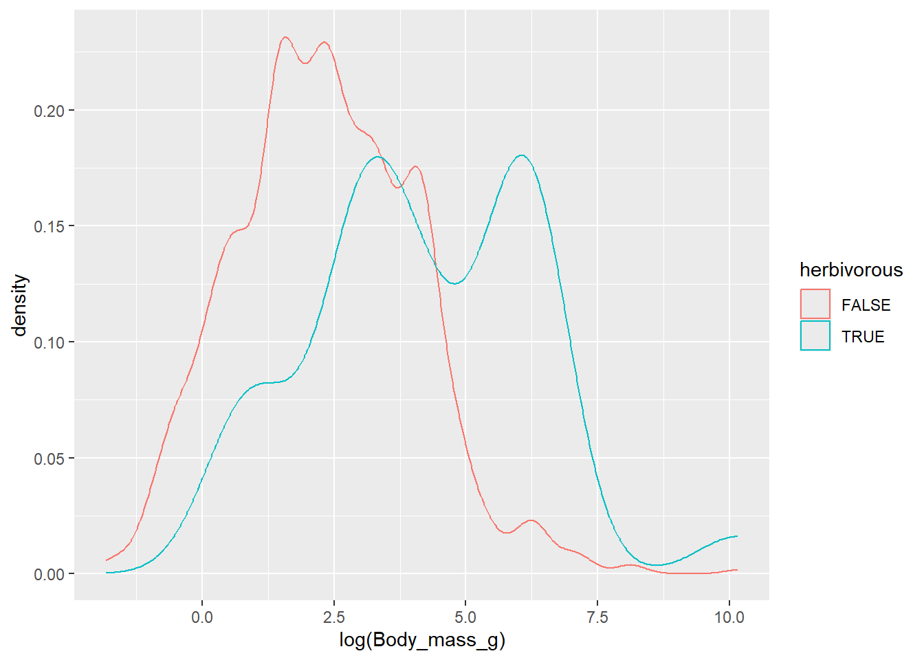

Drought avoidance

One big threat to terrestrial amphibians is desiccation. One would expect that this threat is more immediate in drier climates, and the species in dry systems are thus expected to avoid the day to reduce thermal stress. Do terrestrial amphibians indeed tend to more often be nocturnal/crepuscular (rather than diurnal) in dry climates than in wet climates? Calculate the proportion of species (across all orders) that is diurnal for both climates:

Use the dat dataset, and remove records where the “diel” column is NA;
Compute a new variable, called “isDiurnal”, that is TRUE when it concerns a diurnal species (“Diu”), yet FALSE when it is not diurnal (thus nocturnal “Noc” or crepuscular “Crepu”);
Drop records where the “drywet” column is NA;
Compute the proportion of diurnal species for dry and wet habitats.

dat %>%
  drop_na(diel) %>%
  mutate(isDiurnal = diel == "Diu") %>%
  drop_na(drywet) %>%
  group_by(drywet) %>%
  summarize(propDiu = mean(isDiurnal))

## # A tibble: 2 × 2
##   drywet propDiu
##   <chr>    <dbl>
## 1 Dry      0.272
## 2 Wet      0.243

Bergman’s rule

According to Bergman’s rule, colder environments tend to harbour larger species than warmer regions. Bergman’s rule holds for mammals and birds, which are endotherms. Does the rule also hold for frogs? Compare the distribution of frog (order “Anura”) body mass between warm and cold climates:

Perform the following steps to solve this question:

Subset the dataset dat to Anura (column “Order”) only;
Remove rows in which the “coldwarm” column is NA;
Compute the logarithm of body mass (column “Body_mass_g”) as a new column called “BMlog”;
Compute a new column called “y” that has the value 0.01 for “cold” habitat, and the value 0.02 for “warm” habitat;
Plot a density plot of “BMlog”, where the cold and warm habitats are shown in separate lines with different colours;
Add points to the plot where “BMlog” is the x-coordinate and “y” the y-coordinate of the points;
Add axis labels: “Body mass (log)” on the x-axis, and “Density” on the y-axis.

dat %>%
  filter(Order == "Anura",
         !is.na(coldwarm)) %>%
  mutate(BMlog = log(Body_mass_g),
         y = case_when(coldwarm == "cold" ~ 0.01,
                       coldwarm == "warm" ~ 0.02,
                       TRUE ~ 0)) %>%
  ggplot(mapping = aes(x = BMlog, col=coldwarm)) + 
  geom_density() + 
  geom_point(mapping = aes(y=y)) + 
  xlab("Body mass (log)") + 
  ylab("Density")

r/K strategy

Most amphibians produce large numbers of offspring that are un-nurtured, which is typical for an r-strategy. Some, however, do not. Is there evidence for a negative relationship between clutch size and longevity? To solve this question:

Use the dat dataset, but exclude the Gymnophiona order;
Compute the mean longevity (column “Longevity_max_y”) and mean litter size (column “Litter_size_min_n”) per species (remove NAs in the computation of the means);
Create a scatter plot, with longevity on the x-axis, and litter size on the y-axis;
Make sure that both the x-axis as well as y-axis are on a square-root scale;
Add a linear trend line through the points;
Make a separate panel for the different orders.

dat %>%
  filter(Order != "Gymnophiona") %>%
  group_by(Order, Species) %>%
  summarize(Longevity_max_y = mean(Longevity_max_y, na.rm = TRUE),
            Litter_size_min_n = mean(Litter_size_min_n, na.rm = TRUE)) %>%
  ggplot(mapping = aes(x = Longevity_max_y, y = Litter_size_min_n)) +
  scale_x_sqrt() + 
  scale_y_sqrt() + 
  geom_point() + 
  geom_smooth(method = "lm") +
  facet_wrap(~Order)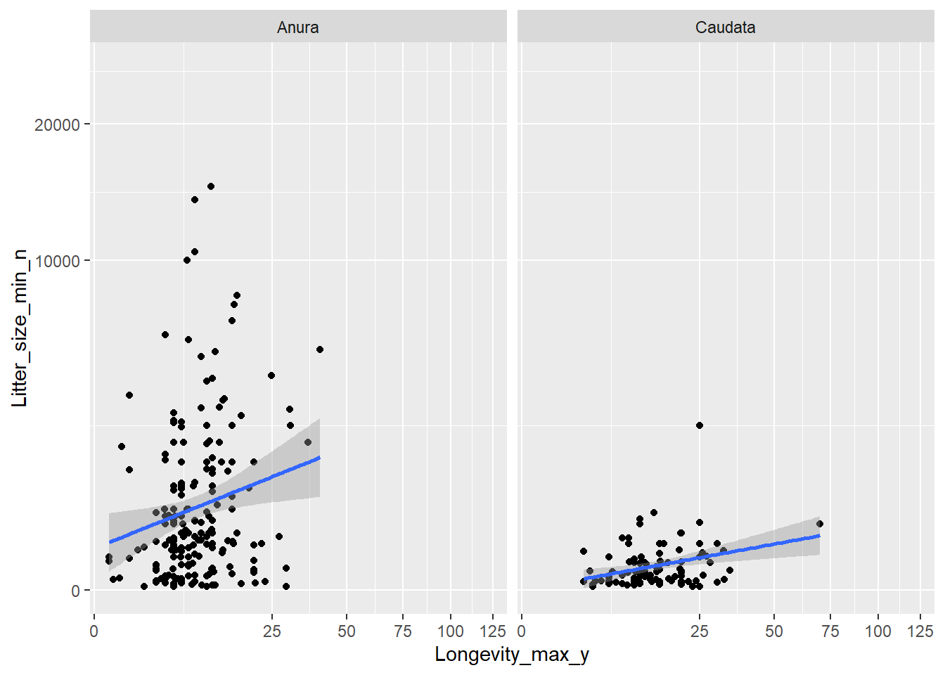

Offspring trade-offs

Resources can be spent only once. One important trade-off that animals and plants therefore face is whether to produce more but smaller offspring or larger but fewer offspring. This trade-off is well documented in seed plants. Does this trade-off also hold for anurans? To solve this question, check how reproductive output of anurans correlates with body size:

Use the dat dataset, subsetted only to the Anura order;
Select only the columns “Species”, “Body_mass_g” and “Reproductive_output_y”;
Compute the mean body mass and reproductive output per species, after log10-transforming them. Call the mean log-body mass “x”, and the mean log-reproductive output “y”;
Create a scatter plot with a linear trend line fitted through the points (with “x” on the x-axis and “y” on the y-axis);
Calculate the Pearson correlation coefficient using the cor function (with method = "pearson" and using only complete observations) and calculate its significance with the cor.test function.

# subset data and compute summaries
dat_sub <- dat %>%
  filter(Order == "Anura") %>%
  select(Species, Body_mass_g, Reproductive_output_y) %>%
  mutate(x = log10(Body_mass_g),
         y = log10(Reproductive_output_y)) %>%
  group_by(Species) %>%
  summarize(x = mean(x, na.rm = TRUE),
            y = mean(y, na.rm = TRUE))

# plot 
dat_sub %>%
  ggplot(mapping = aes(x = x, y = y)) +
  geom_point() +
  geom_smooth(method = "lm")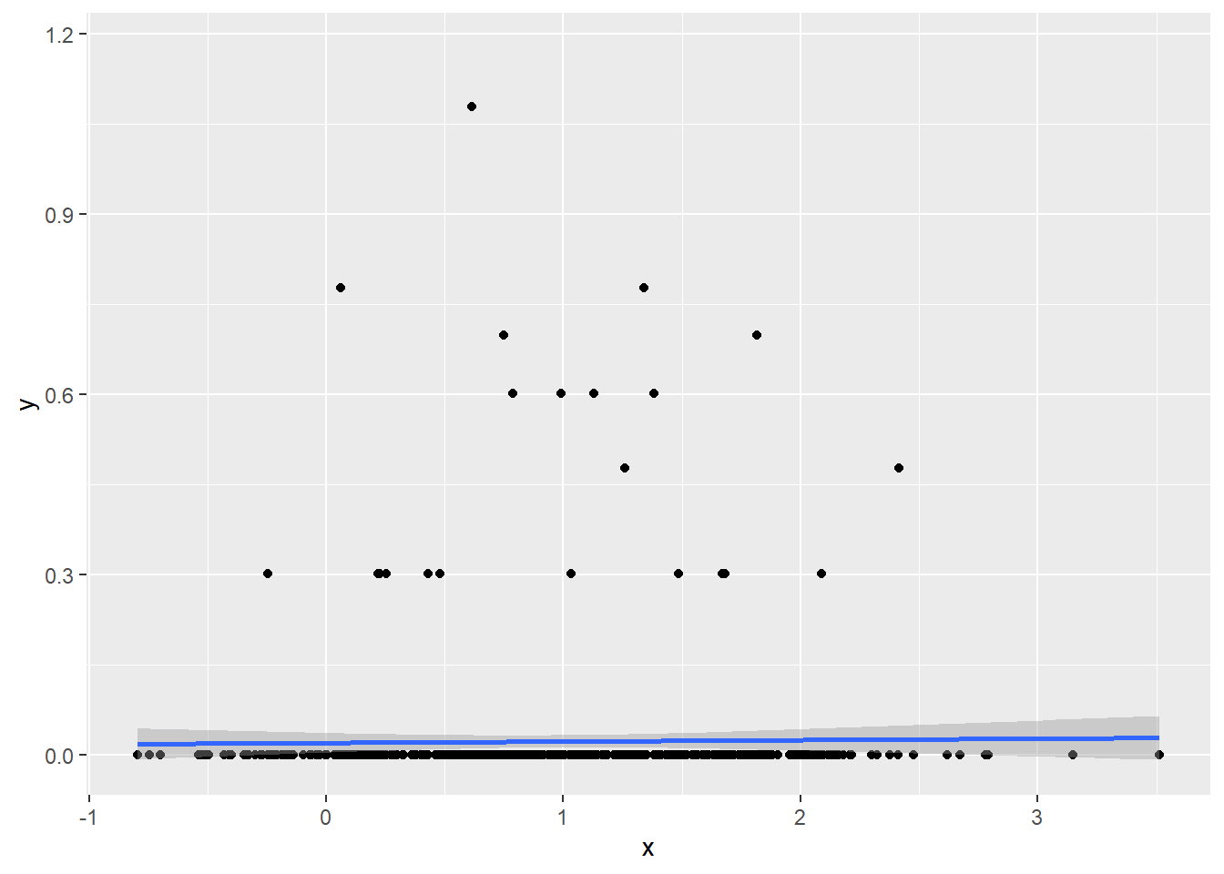

# compute correlations
cor(dat_sub$x, dat_sub$y, use = "complete.obs", method = "pearson")

## [1] 0.0156225

cor.test(dat_sub$x, dat_sub$y, method = "pearson")

## 
##  Pearson's product-moment correlation
## 
## data:  dat_sub$x and dat_sub$y
## t = 0.34017, df = 474, p-value = 0.7339
## alternative hypothesis: true correlation is not equal to 0
## 95 percent confidence interval:
##  -0.07435797  0.10535064
## sample estimates:
##       cor 
## 0.0156225

Tidymodels

Use the tidymodels toolbox to test how well the traits of the species can be used to classify the species to order level.

First:

Use the dat dataset, removing records where the species belongs to the “Gymnophiona” order;
Keep only the “Order” column, and all columns that are numeric;
Drop records that contain NA values;
Convert “Order” into a factor with levels “Anura” and “Caudata”;
Assign the resultant dataset to an object called modelDat.

Then:

create a random split of the modelDat dataset, keeping 60% for training and 40% for testing;
Retrieve the train and test datasets, call them modelDatSplits_Train and modelDatSplits_Test, respectively.

Then:

create a data recipe (called rec), that specifies that the column “Order” is the response, and all other columns in modelDatSplits_Train are predictors;
Scale and center all predictor variables convert all numeric features into principal components, using the appropriate step_... functions. Preserve only 3 principal components;
prepare the data recipe with the train dataset;
bake both the train and test datasets.

Then:

specify a logistic regression model, with “classification” mode and “glm” engine, where “Order” is the response variable and all other columns are predictors;
Fit the specified model on the baked train dataset;
use the fitted model to predict the order in the baked test dataset;
Get the classification metrics.

library(tidymodels)

# Prepare
modelDat <- dat %>%
  filter(Order != "Gymnophiona") %>%
  dplyr::select(Order, where(is.numeric)) %>%
  drop_na() %>%
  mutate(Order = factor(Order, levels = c("Anura","Caudata")))

# Get train/test splits
modelDatSplits <- initial_split(modelDat, prop = 0.6)
modelDatSplits_Train <- training(modelDatSplits)
modelDatSplits_Test  <- testing(modelDatSplits)

# Create data recipe
rec <- recipe(Order ~ ., data = modelDatSplits_Train) %>%
  step_scale(all_predictors()) %>%
  step_center(all_predictors()) %>%
  step_pca(all_numeric(), num_comp = 3)

# prep the data recipe with training data
rec <- rec %>%
  prep(modelDatSplits_Train)

# Bake the datasets
modelDatSplits_TrainBaked = rec %>%
  bake(modelDatSplits_Train)
modelDatSplits_TestBaked = rec %>%
  bake(modelDatSplits_Test)

# Fit logistic regression
modelFit <- logistic_reg(mode = "classification") %>%
  set_engine("glm") %>%
  fit(Order ~ ., data = modelDatSplits_TrainBaked)

# Predict on test set
modelFitData <- modelFit %>% 
  predict(modelDatSplits_TestBaked, type="class") %>%
  bind_cols(modelDatSplits_TestBaked)

# Get metrics
modelFitData %>%
  metrics(truth = Order,
          estimate = .pred_class)

## # A tibble: 2 × 3
##   .metric  .estimator .estimate
##   <chr>    <chr>          <dbl>
## 1 accuracy binary         0.867
## 2 kap      binary         0.687

Appendix C - Test exercises

Introduction

Loading and preparing data

Some exploration of the data

Jarman–Bell principle

Drought avoidance

Bergman’s rule

r/K strategy

Offspring trade-offs

Tidymodels