You can use the load.dir() function from the
imager package to load all images in a directory at once, which
will then return a list of cimg objects.
Preparing images for analyses
Overview
Totday’s goal: prepare image data for the analyses on day 3 of this week.
Resources
1 Introduction
In the tutorials of the next days, you will train and apply a Convolutional Neural Network (CNN) yourself to distinguish bush and trees from grass and bare soil within images. For this you will use the famous Keras package. You will train the CNN and optimize its performance on a separate validation set. Afterwards you will apply the CNN on a new image to see the output of the CNN in practice. Take note that you can tweak a lot to improve its performance: the annotation of your data, the structure of your network and the chosen hyperparameters. This means that you will probably won’t get everything right the first time, but also that there is a lot of room for improvement. Let’s see if you are able to beat our performance!
Image data is by definition not tidy data, because the colour values of each pixel are not independent of the values in the neighbouring pixels. Only by evaluating the pixels combined on a larger scale, does an object or feature in an image become apparent. Therefore, the preprocessing and wrangling of image data looks differently than for tabular data. This is what you will practice today. The day after tomorrow you will then use your prepared data to train and evaluate a CNN. This practical is aimed at learning the imager package.
If you try to install the imager package on a MacBook, and load it after installing it, it may be that you are getting an error. This is most likely caused by an older version of the Xquartz software that is already installed on your system. This error can be solved by updating the Xquartz software, which you can download and install from here.
Exercise 14.1a
Start by downloading the images
(IMG_4012.JPG,IMG_4013.JPG,IMG_4014.JPG)
from Brightspace > Image analyses > Data > Images 1,
save them to a folder named images1 inside data /
raw. To load and mutate the images we need the tidyverse,
imager and abind packages, so install and load these
packages. Furthermore, make sure to set your working directory correctly
again.
cimg objects (i.e., an
imager object) using the function load.image, and
assign the result to an object called im. Then, plot the
images using the base R plot function (this might take a
while to execute). To load the images:
# Load libraries
library(tidyverse)
library(imager)
library(abind)

# Load all images in a directory
im <- load.dir("data/raw/images1")
To plot the images:
# Plot the images
plot(im)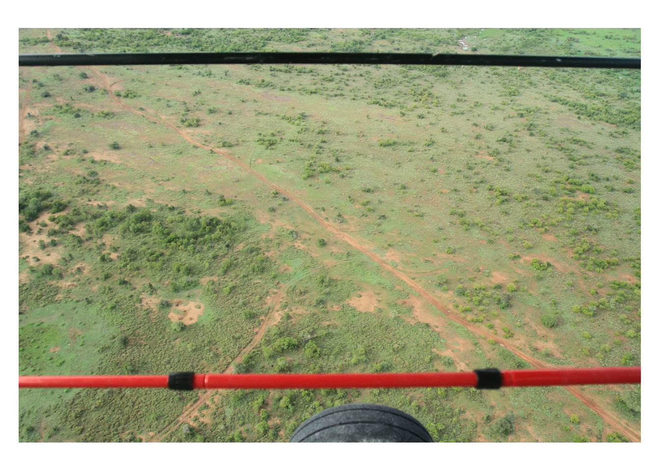


Exercise 14.1b
Inspect the structure of your newly loaded objects using the
str function. What type of R object is cimg
primarily? # explore the im object
str(im)## List of 3
## $ IMG_4012.JPG: 'cimg' num [1:5184, 1:3456, 1, 1:3] 0.557 0.545 0.533 0.561 0.569 ...
## $ IMG_4013.JPG: 'cimg' num [1:5184, 1:3456, 1, 1:3] 0.541 0.545 0.549 0.553 0.557 ...
## $ IMG_4014.JPG: 'cimg' num [1:5184, 1:3456, 1, 1:3] 0.694 0.682 0.69 0.694 0.675 ...
## - attr(*, "class")= chr [1:2] "imlist" "list"You can see that the cimg objects are under the hood
actually arrays. The first two dimensions of the array are the
x and y coordinates of the pixels (5184x3456px in the case of our
images), the third dimension is useful for videos (with multiple frames)
and thus always 1 for pictures, the fourth dimension are the colour
channels of our images (very often three: Red, Green and Blue). Note
that image data is by definition not tidy, as it is a raster of
cells each containing multiple values!
2 Preprocess
As you can see in the plots there are some aircraft parts in view at the top and bottom part of the images.
In some of the exercises below, it is handy to iterate some
piece of R code using a for-loop. A loop is a sequence
of instructions that is repeated a specified number of times, or until a
certain condition is been reached. For instance, the following code uses
a for-loop to iterate some code 10 times, with
iterator object i getting the value 1, 2, …, 10
during these iterations. The R code in this example is very simple: it
solely prints the value of the iterator i to the
console.
for(i in 1:10) {
  print(i)
}
## [1] 1
## [1] 2
## [1] 3
## [1] 4
## [1] 5
## [1] 6
## [1] 7
## [1] 8
## [1] 9
## [1] 10For more information, see Appendix E - Indexing and control structures.
Exercise 14.2a
Cut these parts off to reduce some of the noise in the image. For this
you can use the imsub function from imager. Check
its help page to learn how to define the coordinate range of the image.
Use the same range for every image to make sure that every image still
has the same pixel dimensions. Plot your images again afterwards to
check if you got the range right. If you look very closely you might
also spot some elephants and giraffes. However, being endangered species
and all, you can just leave them roaming around in the images… You can use a for-loop to apply the same transformation on all three images in the list (see Appendix E).
For example, to crop the image to the part between 200 and 500 pixels
from the top you can conveniently use the %inr% operator,
i.e.,: imsub(yourimage, y %inr% c(200,500)).
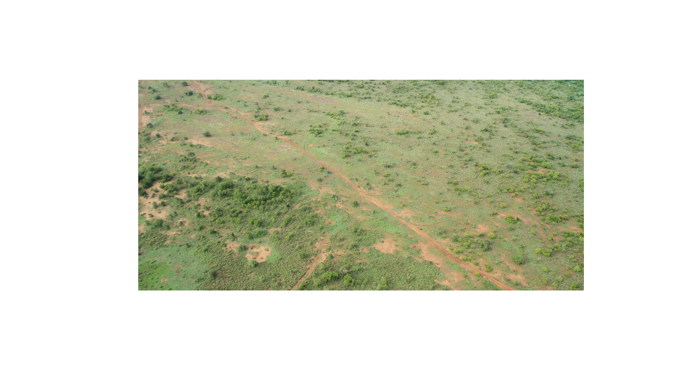
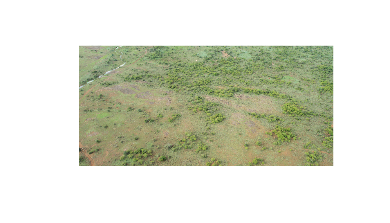
for(i in seq_along(im)) {
  im[[i]] <- imsub(im[[i]], y %inr% c(350,2800))
  plot(im[[i]], axes = FALSE)
}

There are several approaches to distinguish trees from grass in aerial images:
- we could build an object detection algorithm to detect all the trees in the images directly via moving windows and bounding box regression
- we could apply image segmentation to find the boundaries between different vegetation types in the images
- we could divide the images into regular grids and classify each grid cell to be either trees or grass.
In this practical we will apply the third option.
To preprocess our data further to make it ready for analyses, we now need to divide the images into a regular grid where each image is split into multiple tiles.
Exercise 14.2b
In this exercise you are going to divide the images inside the
imlist object into tiles of 50x50 pixels using the
imsplit function and prepare for further analyses. Do this
via the following steps:
- Split the images into 50-pixel bands along the x-axis (thus resulting in vertical bands);
- Remove the last band, as most probably you cannot exactly fit an integer number of bands along the x-axis of your image;
- Split each vertical band into 50-pixel high tiles;
- Remove the bottom row, as most probably this is not 50 pixels high; the remaining tiles are thus all 50x50 pixels;
- Make sure to change the class of both the first and
second level of the original
imlistobject to alist.
If object im is an object of class list or
imlist, then the following code can be used to create a
for-loop that iterates over all images in the list:
for(i in seq_along(im)) {
  # commands to be executed
  im[[i]] # here e.g. retrieving the image from the list at position i
}
If you want to split an image, e.g. im[[i]], into bands
of 250 pixels wide, along the x-axis, you could use:
im[[i]] <- imsplit(im[[i]], axis = 'x', nb = -250)To remove the last element from a list, you could use:
im[[i]] <- im[[i]][-length(im[[i]])]Also, if element im[[i]] is a list itself, you could
retrieve (or set) the element at position j using
im[[i]][[j]].
To specify the class of an object, your
could use the class function. For example, to change the
class of element i of an object im into a
‘list’, you could use:
class(im[[i]]) <- 'list'# A first (outer) for-loop that iterates over the images
for(i in seq_along(im)) {
# Split into 50-pixel bands along x-axis
im[[i]] <- imsplit(im[[i]],
axis = 'x',
nb = -50)
# Remove last band as it most probably will not be 50 pixels wide
im[[i]] <- im[[i]][-length(im[[i]])]
# A second (inner) for-loop that iterates over the image bands created above
for(j in seq_along(im[[i]])) {
# split each band vertically in 50-pixel tiles
im[[i]][[j]] <- imsplit(im[[i]][[j]],
axis = 'y',
nb = -50)
# Remove last band as it most probably will not be 50 pixels high
im[[i]][[j]] <- im[[i]][[j]][-length(im[[i]][[j]])]
}
}
# Convert each element to class 'list'
for(i in seq_along(im)) {
class(im[[i]]) <- 'list'
}
# Convert the entire object to class 'list'
class(im) <- 'list'
Exercise 14.2c
Finally, save the tiles of all three prepared images as PNG files to
a new folder images1 in the data/processed/
folder (thus: data/processed/images1/), using the
save.image function. Do this using the following steps:
- First create three folders in your in your ‘data/processed/images1’ folder, and call them test, train and val.
- Save the tiles of the first list-element in our
im-object (named IMG_4012.JPG) to the test folder; these will be the tiles you will later (in the tutorial on CNN model fitting and evaluation) test your trained image classification model on. Save the tiles in the second list-element (IMG_4013.JPG) to the train folder; these will be used to train the classification model. Save the tiles of the last list-element (IMG_4014.JPG) to the val folder; these will be used for validation. - Name the export files ‘x_y.png’, where ‘x’ should be the
index-position of the tiles in the x dimension and ‘y’ the
index-position of the tiles in the y dimension. Notice this will take a
while to execute, but you can keep track of the progress by looking at
the number of images in the folders in file explorer. In rendering this
document, there were about 5047 files per folder, but this might differ
a bit if you cut off more or less of the image to remove the aircraft
parts.
This is an example code that uses 3 nested for-loops to save all images in the objectimautomatically to some location on your computer:
# Export all 50x50 pixel images (all tiles for 1 image to test/, 1 to train/ and 1 to val/)
for(i in seq_along(im)) {
  folder <- c("test","train","val")[i]
  for(j in seq_along(im[[i]])) {
    for(k in seq_along(im[[i]][[j]])) {
      save.image(im[[i]][[j]][[k]],
                 file = paste0("data/processed/images1/", folder, "/", j, "_", k, ".png"))
    }
  }
}
Why is it good practice to assign entire images to different sets?
It is important to split your dataset into train, validation and test sets as early on in your workflow as possible. Within an image there is spatial autocorrelation between the pixels, so it is good practice to assign the entire image to different sets to avoid overfitting your model.
3 Labelling
Now we move away from R for a while. Don’t be sad: we will be back soon.
Probably the most vital aspect of supervised learning is the availability of labels. Although there are techniques available to automatically generate labels, very often it still up to us to manually label some records. “Some” might actually mean 10,000+ images, but in our case we’ll try to get away with less. However, we still have to roll up our sleeves, put on our glasses and prepare a good coffee, because we have to get to work.
Start by creating two empty folders in both the train
and val folder called bush and
other. Then open another file explorer window, go to the
train/bush folder and drag this window in view next to the
other window with the train root folder opened. First
scroll through our train folder to get a feeling for the
differences in vegetation types. Identifying which cells are trees or
bush is not always straightforward and is actually subjective. Determine
for yourself what you consider to be trees/bush and what
you consider to be grass and other background. Remember that what you
put into your model is what your model learns. GIGO: Garbage
In, Garbage Out. If you tell a very smart model that all dog images are
cats, then that’s what that model will output to you as well.
After you’ve decided what you consider to be bush/trees,
copy (do NOT move/drag, but really copy!) a selection of 50 images of
trees from the train folder to the train/bush
folder. Then afterwards do the same for the validation set. When you’re
done with that we need to select an equal amount of non-tree images to
the other folders. Take into account that your model will only learn
with what you supply it. So if you don’t supply it with images of water
or bare soil, it might give unexpected results for water and bare soil
images if you let the model predict on these images. So try to provide
the model with enough variation in images per class to be
representative for the entire images.
Have fun!
Why is it good practice to assign an equal amount of images to different
classes?
This makes the validation of our model much easier, because we don’t have to deal with class imbalance in the calculation and/or selection of our performance metrics. However, be aware that if you train a model to detect trees in the desert and you supply it with an equal amount of trees and non-tree images during training and validation, it will likely predict too many trees to actual desert images (that do contain much fewer trees).
Exercise 14.3a
When you’re done, load the labelled images into R with the
load.dir function. Call these objects train1
(for train/bush), train0 (for
train/other), val1 (for val/bush)
and val0 (for val/other). Do not load all the
test tiles as well, because this will mess up the order of the tiles and
you already have these data loaded in (inside im[[1]]).
Just convert this multi-level list im[[1]] to a single
imlist and name it testgrid. You can do this
quickly with the do.call function, which executes another
function with a list of arguments (in this case we aim to combine all
the separate list elements into one list). Afterwards make sure to also
convert your testgrid list to an imlist class,
so that imager also recognizes it properly. Then save this object as an
.rds file called “testgrid.rds” to your appropriate data folder, because
we need it later to evaluate our model predictions. # Load train images
train0 <- load.dir("data/processed/images1/train/other")
train1 <- load.dir("data/processed/images1/train/bush")
# Load validation images
val0 <- load.dir("data/processed/images1/val/other")
val1 <- load.dir("data/processed/images1/val/bush")
# Prepare test images
testgrid <- do.call(c, im[[1]])
testgrid <- as.imlist(testgrid)
# Save testgrid
write_rds(testgrid, file = 'data/processed/images1/testgrid.rds')4 Data augmentation
Maybe your mathematics teacher in high school taught you the very valuable lesson that good mathematicians are lazy mathematicians. You’ll be pleased to know that the same applies to data scientists. However, we have an extra trick up our sleeves: not only can we use mathematical principles to do the work for us, also computational power. If we combine these two it can lead to interesting combinations.
More labelled data is always better (even when it’s not, because we
can then still choose to include only a fraction of it), so let’s
generate some labelled data for free. Take a look at the below example,
using a build-in image of the imager package.
par(mfrow = c(1,3)) # defining multiple plot facets: 1 row and 3 columns
plot(boats)
mirror(boats,"x") %>% plot()
mirror(boats,"y") %>% plot()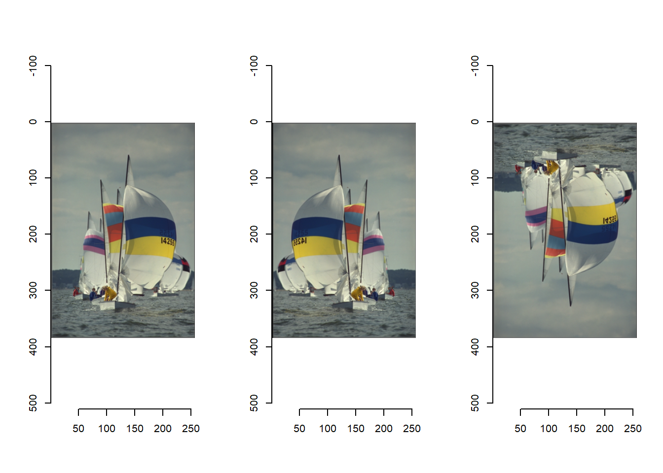
What do you notice about the above plotting example?
Mirroring an image along the x-axis results in a recognizable, real-life image that could in theory have been an actual photograph itself. So we can actually generate twice as much labelled training data by mirroring all our labelled tiles along the x-axis.
Exercise 14.4a
Now use the mirror function to generate x-axis mirrored versions of our
training data for both the ‘bush’ and ‘other’ labels. Store these
mirrored versions in the elements 51 to 100 of our train1
and train0 lists by using a for-loop. for(i in seq_along(train1)) {
train1[[(i+50)]] <- mirror(train1[[i]], "x")
train0[[(i+50)]] <- mirror(train0[[i]], "x")
}
Why don’t we apply data augmentation to the validation or test set?
Augmenting training data is useful, because it can likely result in a model that has learned more and performs better. For the validation and test set this doesn’t apply, because we’re only interested to see how our model performs on the actual data and not on augmented data.
5 Saving data
Exercise 14.5a
In order to easily load the data that you prepared today into your R
session during the tutorial where you will start fitting a CNN
classification model to the image data, save the objects
train0, train1, val0 and
val1 to .rds files (see
tutorial
1) in the “data/processed/images1/” folder. # Save files to rds
write_rds(train0, file = "data/processed/images1/train0.rds")
write_rds(train1, file = "data/processed/images1/train1.rds")
write_rds(val0, file = "data/processed/images1/val0.rds")
write_rds(val1, file = "data/processed/images1/val1.rds")6 Recap
Today, you’ve pre-processed your image data so that it can be used by a CNN. With the tiny images you’ve extracted from the main images, the augmented training data you’ve generated and the class labels you’ve given to some of these images, you now have all the ingredients to train and validate a classification model with these data. This you will do yourself during the final days of the image analysis week, so make sure to properly save your scripts and data.
An R script of today’s exercises can be downloaded here