Reproducible research
Today’s goal: learn to use R markdown in order to facilitate reproducible science.
- R4DS: chapters 27 R Markdown, optionally chapters 28 Graphics for communication, 29 R Markdown formats, and 30 R Markdown workflow
- rmarkdown
- bookdown
- shiny
1 Introduction
In this short tutorial, we will practice creating a report using the R markdown. Markdown is a lightweight markup language with plain-text formatting. Markdown documents can be converted to many other output formats. In Data Science projects, Markdown is often used to format readme files. R Markdown allows to embed R code into Markdown documents.
The typical workflow of creating a document in R markdown consists of six steps:
- Create / open an .Rmd document. In R Studio, this can be done by opening a new R Notebook file (File > New File > R Notebook (R Markdown)), which offers a useful template.
- Write a report in plain text, and use the Markdown syntax to format text
- Write a YAML header that explains what type of document to build from your R Markdown file.
- Use knitr syntax to embed chunks of R code.
- Optionally, embed chunks of Shiny functions for interactive output.
- Use knitr to run the code and render the report with the results embedded.
2 Elephant tracking data
In this tutorial, you will write a report that explains to fellow biologists how a tracking dataset with just two fields of information – timestamp and payload – can be translated into a rich map of locations and trajectories. We will again use the African elephant tracking data collected in Kruger National Park, South Africa, by de Knegt et al. 2011.
This time, however, we have tracks of 2 different individuals.
Download the data file “elephants.csv” from Brightspace > Skills > Datasets > Elephants and store it in a appropriate place.
In the exercises below, you’re asked to write a Markdown report that explained the different steps needed to get to a map of the elephant’s movement tracks. In some exercises, you’re asked to write some text about some steps: it is not meant to write a detailed elaborate text, but rather to practice combining text, code, and output in a single markdown document.
The extra challenge is to also produce a map in a Shiny app that lets the user select individual animals and explore their locations over time using a slider.
–––
title: "Elephant tracks"
author: "Henjo de Knegt"
date:
"`r Sys.Date()`"
output:
html_document:
code_folding:
show
–––
De Knegt and colleagues studied habitat selection by
African elephants in Kruger National Park (KNP), South Africa’s largest
nature reserve, covering roughly 19,000 km2 and harbouring
close to 14,000 African elephants (Loxodonta africana). 33
elephants (19 females and 14 males) were tagged with GPS collars.
Locations were recorded at hourly intervals over a three‐year period
(2005–2008). In this report, I show how R can be used to decipher and
the coded GPS records and be visualized on a map, using a subset of the
data of a subset of individuals.
```{r echo=TRUE, eval=TRUE, warning=FALSE,
include=FALSE}
library(tidyverse)
library(lubridate)
source("https://wec.wur.nl/dse/-scripts/hex2integer.r ")
dat
<- read_csv("data/raw/elephants/elephants.csv")
```
The dataset
that I used contains tracking data from `r length(unique(dat$id))`
individuals, with `r length(dat$id)` fixes in total. Each fix consists
of 3 variables: one number (column _timestamp_) and two strings (columns
_id_ and _payload_).
Datetime objects are often stored in a UNIX timestamp format: a
number that represents the number of seconds that passed since midnight
of January 1, 1970, GMT time. With the package **lubridate**, these
numbers can easily be converted into readable dates and times. Here we
save them as new variable _dttm_.
```{r echo = TRUE, eval =
TRUE}
dat <- dat %>%
mutate(dttm =
parse_date_time("1970-1-1 0:0:00",
orders = "%Y-%m-%d
%H:%M:%S",
tz = "GMT") +
timestamp)
dat
```
The payload is a text string composed of a series of codes, called
nibbles.
1. The first 4 nibbles codes for the ambient temperature
* 10
2. The second 7 nibbles codes for the GPS longitude * 1e5
3.
The last 7 nibbles code for the GPS latitude * 1e5
Using the
`str_sub` function, we can break up the payload string as
follows:
```{r echo = TRUE, eval = TRUE}
dat <- dat
%>%
mutate(temp_hex = str_sub(payload, start = 1, end =
4),
lon_hex = str_sub(payload, start = 5, end =
11),
lat_hex = str_sub(payload, start = 12, end = 18))
%>%
select(-c(timestamp,payload))
dat
```
Then, to
make clear that these are not numeric data, we add the prefix *0x*, as
follows.
```{r echo = TRUE, eval = TRUE}
dat <- dat
%>%
mutate(temp_hex = str_c("0x",temp_hex,sep=""),
lon_hex = str_c("0x",lon_hex,sep=""),
lat_hex =
str_c("0x",lat_hex,sep=""))
dat
```
The last step consists of converting the hexadecimal codes to
integers and divide these by 1e5, to obtain latitude and longitude.
```{r echo = TRUE, eval = TRUE}
dat <- dat
%>%
mutate(lon = map_dbl(lon_hex, hex2integer) /
1e5,
lat = map_dbl(lat_hex, hex2integer) /
1e5)
dat
```
addPolylines(lng=~lon, lat=~lat).
Now that we have converted the data from hexadecimal representation
into decimal representation, we can plot the elephant trajectories on a
dynamic `leaflet` map, plotting a separate line for each individual. We
will also show different base layers: the default open-streetmap layer,
as well as the ESRI world imagery data. We will add a menu where you can
toggle the individuals as well as the base layer.
```{r echo =
TRUE, eval = TRUE}
library(leaflet)
leaflet(dat)
%>%
addTiles(group = "default") %>%
addTiles(urlTemplate
=
"server.arcgisonline.com/ArcGIS/rest/services/World_Imagery/MapServer/tile/{z}/{y}/{x}.png",
attribution = "ESRI world imagery",
group = "ESRI world
imagery") %>%
# Add separate lines
addPolylines(lng = ~lon,
lat = ~lat, color = "#ff0000", group = "am72",
data =
filter(dat, id == "am72")) %>%
addPolylines(lng = ~lon, lat =
~lat, color = "#0000ff", group = "am160",
data =
filter(dat, id == "am160")) %>%
# Layers
control
addLayersControl(
baseGroups = c("default", "ESRI
world imagery"),
overlayGroups = c("am72",
"am160"),
options = layersControlOptions(collapsed =
FALSE)
)
```
The map shows …
If you want to export markdown documents in pdf format, it may be
needed to install and load the package TinyTeX and then
run the code tinytex::install_tinytex() (or install another
LaTeX distribution, e.g. MikTex). Some contents, e.g. the leaflet map as
produced above, are intrinsically html/javascript based, so documents
with such contents will have problems rendering to pdf. For more
information, see
here.
However, in such cases you can use the
webshot
package, which makes it easy to take screenshots of web pages and other
content from R, thus even when exporting to pdf, html content can still
be included!
See this site for a html rendered version of the report as shown above.
3 Challenge
Create a shiny app with the map of the locations that allows users (a) choose which individual to display, through a button, (b) to trace the location of the animal at any given time, through a slider, and (c) both combined.
The shiny homepage and cheat sheets can be found at the top of this page.If you want, you can also submit a printscreen of your shiny app, or host it somewhere (e.g. via www.shinyapps.io) and share a link.
Given the resultant tibble dat as produced with the code
above, the code to produce a very simple Shiny app with the
data from this tutorial could look like this:
# Prelims
library(tidyverse)
library(shiny)

# data: object `dat` as preprocessed above

# Preprocess dataset dat further:
# convert id to factor and ge nr of rows
dat <- dat %>%
  mutate(id = as.factor(id)) %>%
  group_by(id) %>%
  mutate(nr = row_number()) %>%
  ungroup()

# Get range of lon/lat values
xlims <- range(dat$lon)
ylims <- range(dat$lat)

# Get nr of records for each id, to influence the shiny controls
nrRecordsMax <- max(c(nrow(filter(dat,
                                  id == "am72")),
                      nrow(filter(dat,
                                  id == "am160"))))

# Specify user interface
ui <- fluidPage(
  checkboxGroupInput(inputId  = "whichanimal",
                     label    = "Show animal",
                     choices  = list("am72","am160"),
                     selected = c("am72","am160")),
  sliderInput(inputId = "slider",
              label = "Show record",
              min = 1, max = nrRecordsMax,
              value = 300),
  sliderInput(inputId = "trailsize",
              label = "Size of trails",
              min = 0, max = 500,
              value = 300),
  sliderInput(inputId = "pntsize",
              label = "Size of points",
              min = 0, max = 4,
              value = 1),
  plotOutput(outputId = "plotid")
)

# Set up server function
server <- function(input, output) {
    output$plotid <- renderPlot({
      dat %>%
        filter(nr <= input$slider,
               nr >= (input$slider - input$trailsize),
               id %in% input$whichanimal) %>%
        ggplot(aes(x = lon,  y = lat,
                   group = id, col = id)) +
        xlab("longitude") +
        xlim(xlims) +
        ylab("latitude") +
        ylim(ylims) +
        coord_fixed() +
        geom_path() +
        geom_point(size = input$pntsize)
      })
}

# Combine user interface and server function in app
shinyApp(ui = ui, server = server)
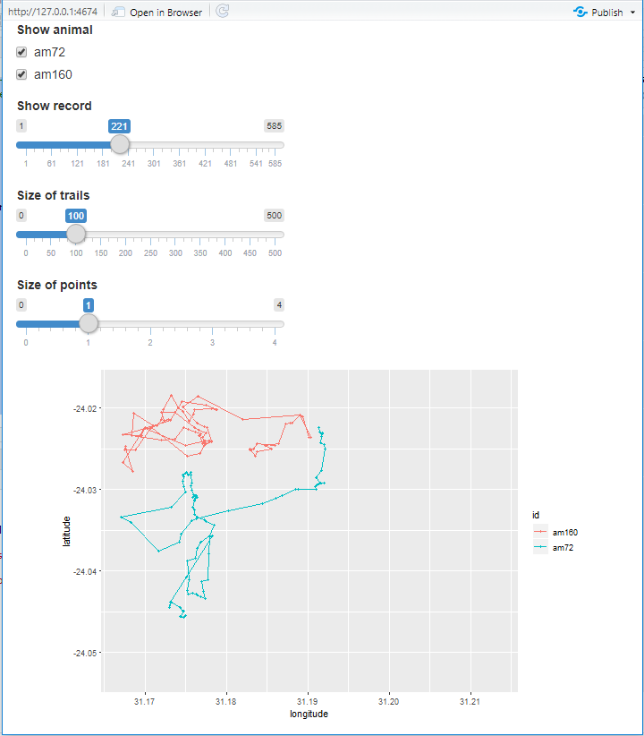
This is a screenshot of the app:
4 Submit your last plot
Submit the .html and the .rmd file of your markdown reaport to Brightspace (Assignments > Skills day 10).
Submit your script file as well as a plot: either your last created plot, or a plot that best captures your solution to the challenge. Submit the files on Brightspace via Assessment > Assignments > Skills day 10.
Note that your submission will not be graded or evaluated. It is used only to facilitate interaction and to get insight into progress.
5 Recap
Today we’ve explored making reproducible reports using RMarkdown.
The resultant RMarkdown script of today’s exercises can be downloaded here.