Use summarise() in combination with n(),
which gives the current group size.
Data wrangling using dplyr
Overview
Today’s goal: to get used to the basic grammar for efficient data transformation using the dplyr package, part of Tidyverse.
Resources
- R4DS: chapters 3
- Data Carpentry - working with data
Packages
Main functions
select, filter, arrange, mutate, summarise, group_by
Cheat sheets
1 Key dplyr functions
Today, we will practice with the package dplyr,
which provides a grammar of data manipulation, and a consistent set of
verbs that help you solve the most common data manipulation challenges.
dplyr provides five main functions for manipulating and transforming
data. These functions – also called verbs – can all be
applied to groups, using group_by:
| Function | Description |
|---|---|
select |
picks variables (columns) based on their names |
filter |
picks cases (rows) based on values of variables |
arrange |
changes the ordering of the rows |
mutate |
generates new variables from existing ones |
summarise |
reduces groups of values into summaries |
group_by |
organizes tibbles in groups |
The first five functions can all be used in conjunction with
group_by, which changes the scope of each function from
operating on the entire dataset to operating on it group-by-group.
Together, these six functions provide the main verbs for a language of
data manipulation.
All verbs work similarly:
- The first argument contains the data: a data.frame or tibble;
- The subsequent arguments describe what to do with the data, using the variable names (without quotes);
- The result is a new data.frame/tibble.
Together these properties make it easy to chain together multiple simple steps to achieve a complex result; this will be dealt with tomorrow.
2 Hoge Veluwe data
We will explore a dataset with observations of wildlife photographed by a permanent array of camera traps installed at National Park De Hoge Veluwe, 20 km Northeast of Wageningen Campus. We use twelve months’ worth of observations (August 2013 - July 2014). The data are part of a project by Patrick Jansen, Yorick Liefting and Jan den Ouden.
The camera-trap array has 48 stations (Reconyx HC500 camera traps mounted at 70 cm height). Eight cameras were placed at random points in each of six mayor habitat types, with half of the points located in restricted area (no access to visitors) and the other half in publicly accessible habitat. Each station received a new deployment (a run with a new memory card and new batteries) every ca. 5 weeks.
The project focuses on five ungulate species – Red deer (Cervus elaphus), Roe deer (Capreolus capreolus), Fallow deer (Dama dama) Wild boar (Sus scrofa) and Mouflon (Ovis ammon musimon). In this tutorial, we will not use the raw data, but data that is already preprocessed and thus in tidy format, with the following files:
| File | Description |
|---|---|
| NPHV_observations_joined.csv | All 27373 observations with joined data |
| NPHV_deer_month_station.csv | The counts of Red deer by month and station |
Exercise 3.2a
Download the files from Brightspace > Skills > Datasets >
NPHV and save them in the appropriate directory! For example, put
the data in the folder data/raw/nphv/; see section
File
management. Load the tidyverse package, and load the file
“NPHV_observations_joined.csv” into a tibble called obs.
library(tidyverse)
obs <- read_csv("data/raw/nphv/NPHV_observations_joined.csv")
3 Creating summaries
With the summarise or summarize functions
(they are synonyms), you can reduce groups of values into summary
statistics. By default: all records in the tibble belong to the same
group (but later we will see how group_by can be used in
conjunction with summarise).
The default syntax for summarise is:
summarise(<data>, <...>)where <data> is the data.frame or tibble
containing the data, and <...> contains the
name-value pairs of summary functions. The specified name will
be used as the name of the variable (column) in the resultant table. The
value can be:
- A vector of length 1, e.g.
min(),n(), orsum(is.na()); - A vector of length n, e.g.
quantile(); - A data.frame/tibble, to add multiple columns from a single expression.
For example, the following command computes the mean of column named
y from dataset x, assigning it the name
meanY:
summarize(x, meanY = mean(y))
Exercise 3.3a
Calculate the total number of observations in obs, and give
it a clear and meaningful name. summarise(obs, nrObservations = n())## # A tibble: 1 × 1
## nrObservations
## <int>
## 1 27373
Exercise 3.3b
Calculate the total number of animals recorded, and give it a clear and
meaningful name. Note that the field “Count” has the number of animals
per observation. Use summarise() in combination with
sum().
summarise(obs, nrAnimals = sum(Count))## # A tibble: 1 × 1
## nrAnimals
## <dbl>
## 1 56366Note that the summary function in base R does not
provide totals: check both summary(obs) and
summary(obs$Count) for yourself.
4 Summaries per group
The function group_by can be used to group records
together, so that summary statistics can be computed per group instead
of across the entire dataset.
The default syntax for group_by is:
group_by(<data>, <...>)where <data> is the data.frame or tibble
containing the data, and <...> contains the grouping
variables. When grouping by multiple variables, they are separated by a
comma. For example, the following command groups the data by the unique
combinations of data in columns y1 and y2 from
dataset x:
group_by(x, y1, y2)In and of itself, the group_by function is only useful
when combining it with other verbs, e.g., summarize.
Exercise 3.4a
Calculate the number of animals recorded per species. Note that the
field “Count” has the number of animals per observation. Use summarise() in combination with sum()
and group_by().
summarise(group_by(obs, Species), nrAnimals = sum(Count))## # A tibble: 28 × 2
## Species nrAnimals
## <chr> <dbl>
## 1 Alauda arvensis 4
## 2 Alopochen aegyptiacus 2
## 3 Bird sp 5
## 4 Blank 2920
## 5 Buteo buteo 4
## 6 Canis lupus familiaris 12
## 7 Capreolus capreolus 2968
## 8 Cervus dama 8
## 9 Cervus elaphus 24472
## 10 Columba palumbus 2
## # ℹ 18 more rows
Exercise 3.4b
Calculate the number of animals recorded per species per habitat. Note
that the field “Count” has the number of animals per observation. summarise(group_by(obs, Species, Habitat), nrAnimals = sum(Count))## # A tibble: 108 × 3
## # Groups: Species [28]
## Species Habitat nrAnimals
## <chr> <chr> <dbl>
## 1 Alauda arvensis Pasture 2
## 2 Alauda arvensis Wet Heathland 2
## 3 Alopochen aegyptiacus Pasture 2
## 4 Bird sp Wet Heathland 5
## 5 Blank Driftsand 148
## 6 Blank Dry Heathland 359
## 7 Blank Forest Culture 330
## 8 Blank Pasture 1145
## 9 Blank Pine Forest 521
## 10 Blank Wet Heathland 417
## # ℹ 98 more rowsIf the group_by function is used, the resultant tibble
contains information on the grouping columns (for details see
here).
Sometimes, the grouping is only an intermediate step in the
transformation pipeline. For example, it may be that we want to compute
new features per group (using the mutate function) or
compute summaries per group (using the summarise function),
and after this step it may be needed to remove the grouping information.
Removing grouping information can be done in different ways. First,
there is the general ungroup function which removes any
grouping information in a tibble. Also, when grouping data and then
summarizing it (using the summarise function), we can use
the (at this stage still experimental) function argument
.groups; see the helpfile of ?summarise. When
setting .groups = "drop", the grouping information is
dropped from the result, yet when setting .groups = "keep"
all grouping information is kept. In many situations, the
summarise function will, by default, drop the last grouping
key (.groups = "drop_last"), potentially having
consequences for subsequent analyses! Namely, if there are 2 or more
grouping columns, then a applying the summarise function
will result in a grouped tibble with all but the last grouping column
maintained, hence any further data transformation will be done on the
resultant groups independently!
5 Arranging rows
The arrange function orders the rows of a
data.frame/tibble by the values of selected columns. Its basic syntax
is:
arrange(<data>, <...>)where <data> is the data.frame or tibble
containing the data, and <...> contains the
variables, or functions of variables, to use for arranging the rows. By
default, values are arranged in ascending order, but by using function
desc you can specify a descending order. The following
command arranges the rows of dataset x based on increasing
values first in column y1, and within that in column
y2:
arrange(x, y1, y2)Note that arrange thus only alters the ordering of the
rows: all data will be preserved, and all variables (i.e., columns)
associated to each record (i.e., row) will stay together.
Exercise 3.5a
Sort rows in obs by columns “Station_ID” and “Month”.
Use arrange().
arrange(obs, Station_ID, Month)## # A tibble: 27,373 × 13
## Month Station_ID Habitat Restricted Camera_Deployment_ID Image_Sequence_ID Image_Sequence_DateTime Observation_ID Count Species Animal_Sex Animal_Age Class
## <dbl> <chr> <chr> <dbl> <dbl> <dbl> <chr> <dbl> <dbl> <chr> <chr> <chr> <chr>
## 1 1 H1R0-01 Driftsand 0 213 10290 01/01/2014 16:03 13593 4 Homo sapie… Unknown Unknown Peop…
## 2 1 H1R0-01 Driftsand 0 213 10293 08/01/2014 16:50 13596 2 Homo sapie… Unknown Unknown Peop…
## 3 1 H1R0-01 Driftsand 0 213 10305 20/01/2014 15:10 13608 1 Setup Pick… Unknown Unknown Other
## 4 1 H1R0-01 Driftsand 0 269 12245 20/01/2014 15:11 15523 1 Setup Pick… Unknown Unknown Other
## 5 2 H1R0-01 Driftsand 0 269 12247 01/02/2014 18:20 15525 1 Homo sapie… Female Sub-Adult Peop…
## 6 2 H1R0-01 Driftsand 0 269 12251 02/02/2014 15:14 15529 2 Homo sapie… Male Adult Peop…
## 7 2 H1R0-01 Driftsand 0 269 12254 05/02/2014 17:13 15532 1 Homo sapie… Male Adult Peop…
## 8 2 H1R0-01 Driftsand 0 269 12254 05/02/2014 17:13 15532 1 Homo sapie… Female Adult Peop…
## 9 2 H1R0-01 Driftsand 0 269 12269 14/02/2014 06:03 15547 1 Blank Unknown Unknown Other
## 10 2 H1R0-01 Driftsand 0 269 12277 16/02/2014 14:30 15555 1 Homo sapie… Female Adult Peop…
## # ℹ 27,363 more rows
Exercise 3.5b
Sort rows in obs by columns “Station_ID” and “Month” , but
now with “Month” in descending order Use arrange() and desc().
arrange(obs, Station_ID, desc(Month))## # A tibble: 27,373 × 13
## Month Station_ID Habitat Restricted Camera_Deployment_ID Image_Sequence_ID Image_Sequence_DateTime Observation_ID Count Species Animal_Sex Animal_Age Class
## <dbl> <chr> <chr> <dbl> <dbl> <dbl> <chr> <dbl> <dbl> <chr> <chr> <chr> <chr>
## 1 12 H1R0-01 Driftsand 0 158 8942 03/12/2013 09:41 12262 1 Setup Pick… Unknown Unknown Other
## 2 12 H1R0-01 Driftsand 0 213 10272 03/12/2013 09:44 13575 1 Setup Pick… Unknown Unknown Other
## 3 12 H1R0-01 Driftsand 0 213 10278 10/12/2013 09:30 13581 1 Cervus ela… Female Adult Mamm…
## 4 11 H1R0-01 Driftsand 0 103 7180 02/11/2013 08:16 10581 1 Capreolus … Male Adult Mamm…
## 5 11 H1R0-01 Driftsand 0 103 7181 08/11/2013 13:57 10582 1 Homo sapie… Male Adult Peop…
## 6 11 H1R0-01 Driftsand 0 103 7182 11/11/2013 14:09 10583 1 Setup Pick… Unknown Unknown Other
## 7 11 H1R0-01 Driftsand 0 158 8938 11/11/2013 14:11 12258 2 Setup Pick… Unknown Unknown Other
## 8 11 H1R0-01 Driftsand 0 158 8941 30/11/2013 14:19 12261 1 Setup Pick… Unknown Unknown Other
## 9 10 H1R0-01 Driftsand 0 56 4592 05/10/2013 19:35 8027 13 Cervus ela… Unknown Unknown Mamm…
## 10 10 H1R0-01 Driftsand 0 56 4595 05/10/2013 19:44 8030 1 Cervus ela… Male Sub-Adult Mamm…
## # ℹ 27,363 more rows6 Filtering rows
The filter function is used to subset a data.frame or
tibble, retaining all rows that satisfy a certain condition. To be
retained, the row must produce a value of TRUE for all
conditions. Note that when a condition evaluates to NA the
row will be dropped. Its basic syntax is:
filter(<data>, <...>)where <data> is the data.frame or tibble
containing the data, and <...> contains the
expression(s) that return a logical value (i.e., TRUE or
FALSE), and are defined in terms of the variables in
<data>.
If multiple expressions are included, they are combined with the
& operator.
For example, the following command filters the rows of dataset
x based on the value in column y1 being equal
to (==) 5, and the value in column y2 being
larger than (>) 100:
filter(x, y1 == 5, y2 > 100)As mentioned above, when separating different logical expressions
using comma, dplyr will assume you mean the logical operator
&. Thus, in this example the following code (the only
difference is that we changed the comma into a & sign)
produces identical output:
filter(x, y1 == 5 & y2 > 100)If you do not want to combine multiple conditional expression via the
& operator (i.e. separated by a comma in the
filter function), you can use the “OR” operator
| instead: for example, if you want to select those rows
from x where either the variable y1
has the value 5, or the variable y2 has a value
that is larger than 100, you could write:
filter(x, y1 == 5 | y2 > 100)
Exercise 3.6a
Filter the observations of Red deer (“Cervus elaphus”) Use filter().
The following retrieves all 12020 observations of Red deer:
filter(obs, Species == "Cervus elaphus")## # A tibble: 12,020 × 13
## Month Station_ID Habitat Restricted Camera_Deployment_ID Image_Sequence_ID Image_Sequence_DateT…¹ Observation_ID Count Species Animal_Sex Animal_Age Class
## <dbl> <chr> <chr> <dbl> <dbl> <dbl> <chr> <dbl> <dbl> <chr> <chr> <chr> <chr>
## 1 8 H6R1-04 Pasture 1 47 3851 01/08/2013 01:04 7287 1 Cervus… Male Adult Mamm…
## 2 8 H6R1-04 Pasture 1 47 3854 01/08/2013 01:15 7290 1 Cervus… Male Adult Mamm…
## 3 8 H6R1-05 Pasture 1 48 3806 01/08/2013 03:01 7242 3 Cervus… Male Adult Mamm…
## 4 8 H6R1-05 Pasture 1 48 3815 01/08/2013 03:21 7251 1 Cervus… Male Sub-Adult Mamm…
## 5 8 H6R1-05 Pasture 1 48 3816 01/08/2013 03:36 7252 1 Cervus… Male Adult Mamm…
## 6 8 H6R1-01-V03 Pasture 1 44 2774 01/08/2013 05:06 6210 1 Cervus… Male Adult Mamm…
## 7 8 H6R1-01-V03 Pasture 1 44 2774 01/08/2013 05:06 6210 3 Cervus… Female Unknown Mamm…
## 8 8 H3R0-01 Dry Heathland 0 5 113 01/08/2013 05:56 3596 2 Cervus… Male Adult Mamm…
## 9 8 H5R1-04 Forest Cultu… 1 38 1891 01/08/2013 06:00 5328 2 Cervus… Male Adult Mamm…
## 10 8 H5R1-04 Forest Cultu… 1 38 1894 01/08/2013 06:08 5331 2 Cervus… Male Adult Mamm…
## # ℹ 12,010 more rows
## # ℹ abbreviated name: ¹Image_Sequence_DateTime
Exercise 3.6b
Filter the observations of Red deer (“Cervus elaphus”) from one station
“H6R1-02” filter(obs,
Species == "Cervus elaphus",
Station_ID == "H6R1-02")## # A tibble: 497 × 13
## Month Station_ID Habitat Restricted Camera_Deployment_ID Image_Sequence_ID Image_Sequence_DateTime Observation_ID Count Species Animal_Sex Animal_Age Class
## <dbl> <chr> <chr> <dbl> <dbl> <dbl> <chr> <dbl> <dbl> <chr> <chr> <chr> <chr>
## 1 8 H6R1-02 Pasture 1 45 3348 04/08/2013 04:49 6784 1 Cervus elaph… Male Adult Mamm…
## 2 8 H6R1-02 Pasture 1 45 3354 04/08/2013 04:53 6790 1 Cervus elaph… Male Adult Mamm…
## 3 8 H6R1-02 Pasture 1 45 3388 06/08/2013 02:07 6824 1 Cervus elaph… Male Adult Mamm…
## 4 8 H6R1-02 Pasture 1 45 3393 06/08/2013 04:05 6829 1 Cervus elaph… Male Adult Mamm…
## 5 8 H6R1-02 Pasture 1 45 3410 06/08/2013 22:49 6846 1 Cervus elaph… Male Adult Mamm…
## 6 8 H6R1-02 Pasture 1 45 3412 06/08/2013 23:45 6848 2 Cervus elaph… Male Adult Mamm…
## 7 8 H6R1-02 Pasture 1 45 3430 06/08/2013 23:52 6866 2 Cervus elaph… Male Adult Mamm…
## 8 8 H6R1-02 Pasture 1 45 3437 06/08/2013 23:57 6873 2 Cervus elaph… Male Adult Mamm…
## 9 8 H6R1-02 Pasture 1 45 3438 08/08/2013 03:07 6874 2 Cervus elaph… Male Adult Mamm…
## 10 8 H6R1-02 Pasture 1 45 3468 11/08/2013 00:11 6904 1 Cervus elaph… Male Adult Mamm…
## # ℹ 487 more rowsThis is equivalent to:
filter(obs, Species == "Cervus elaphus" & Station_ID == "H6R1-02")
Exercise 3.6c
Filter the observations of Wild boar (“Sus scrofa”) that concern more
than 10 individuals
filter(obs, Species == "Sus scrofa", Count > 10)## # A tibble: 22 × 13
## Month Station_ID Habitat Restricted Camera_Deployment_ID Image_Sequence_ID Image_Sequence_DateT…¹ Observation_ID Count Species Animal_Sex Animal_Age Class
## <dbl> <chr> <chr> <dbl> <dbl> <dbl> <chr> <dbl> <dbl> <chr> <chr> <chr> <chr>
## 1 8 H6R0-01 Pasture 0 41 2569 06/08/2013 21:25 6005 12 Sus sc… Unknown Juvenile Mamm…
## 2 9 H6R1-01-V03 Pasture 1 93 6100 10/09/2013 14:18 9501 11 Sus sc… Unknown Juvenile Mamm…
## 3 9 H6R1-01-V03 Pasture 1 93 6103 10/09/2013 14:42 9504 11 Sus sc… Unknown Juvenile Mamm…
## 4 4 H6R1-01-V03 Pasture 1 371 16824 01/04/2014 04:23 20089 16 Sus sc… Unknown Juvenile Mamm…
## 5 4 H5R1-01 Forest Cultu… 1 358 15309 13/04/2014 20:17 18574 15 Sus sc… Unknown Juvenile Mamm…
## 6 5 H6R1-03 Pasture 1 415 20148 02/05/2014 23:30 23413 13 Sus sc… Unknown Juvenile Mamm…
## 7 5 H6R1-01-V03 Pasture 1 424 20267 07/05/2014 00:09 23532 13 Sus sc… Unknown Juvenile Mamm…
## 8 5 H6R0-02 Pasture 0 422 19506 17/05/2014 22:03 22771 11 Sus sc… Unknown Juvenile Mamm…
## 9 5 H6R0-02 Pasture 0 422 19621 24/05/2014 23:22 22886 17 Sus sc… Unknown Juvenile Mamm…
## 10 5 H6R0-02 Pasture 0 422 19652 26/05/2014 05:57 22917 12 Sus sc… Unknown Juvenile Mamm…
## # ℹ 12 more rows
## # ℹ abbreviated name: ¹Image_Sequence_DateTime
Exercise 3.6d
filter the data based on non-animal records in “Species”. Some records of the dataset
obs contain observations that were
not actually from animals. For example, the column “Species” contains
not exclusively animal species names, but also the values: “Unknown”,
“Homo sapiens”, “Skipped”, “Setup Pickup”, “Blank”, and “Park Staff”.
Moreover, when there were animals on the images, not always was the
distinction between male or female clear, so that the column
“Animal_Sex” also the value “Unknown” contains. Subset the dataset
obs to exclude these non-animal entries in “Species”, as
well as to exclude the animals with unknown sex. How many male and
female animals remain in the dataset? i.e.: what is the sum of “Count”
of the filtered dataset per sex? Check ?'==', ?'%in%',
?'&', ?'|' and ?'!'
obssub <- filter(obs,
                 Animal_Sex != "Unknown" &
                   ! Species %in% c("Unknown","Homo sapiens",
                                    "Skipped","Setup Pickup",
                                    "Blank","Park Staff"))
summarise(group_by(obssub, Animal_Sex),
          sum = sum(Count))
## # A tibble: 2 × 2
## Animal_Sex sum
## <chr> <dbl>
## 1 Female 12262
## 2 Male 218317 Selecting columns
The select function is used to select variables in a
data.frame/tibble. The select function makes it easy to
refer to variables based on their name, and allows to select a range of
variables in a concise way: e.g. when the columns of a tibble are named
“a”, “b”, …, “z”, you can easily select the columns “a” till “f” using
a:f (as if they are positions in a vector/data.frame).
Moreover, the select function allows you to use
select_helpers to select variables by matching patterns
in their names (e.g. see ?tidyselect::select_helpers for
more information), or based on their data type (e.g. numeric,
character). The basic syntax of the select function is:
select(<data>, <...>)where <data> is the data.frame or tibble
containing the data, and <...> contains one or more
unquoted expressions separated by commas. The data returned is in the
column-ordering as specified in these expressions. For example, this
code:
select(x, g, a:c, f)selects the columns “g”,“a”,“b”,“c”, and “f” (with those names and in
that order) from dataset x.
Different ways to select variables based on their name(s):
- name without quotes: e.g.,
a(column with name “a”); - a range: e.g.,
a:c(here thus selecting columns “a”, “b” and “c”); - a number: e.g.,
4:6(here thus selecting the 4th, 5th and 6th columns);
Including a minus sign will drop those variables from the dataset, e.g.:
-awill drop column “a”;-(a:c)will drop columns “a”, “b” and “c”;- similarly, column position indices can be used, e.g.,
-1or-(1:3)will drop, respectively, the first column, or the first 3 columns.
See the helpfile of select for the tidy-select
helper functions, e.g.: starts_with,
ends_with, contains, matches and
num_range.
Exercise 3.7a
Load the file “NPHV_deer_month.csv” into a tibble with the name
deer. Select the columns “Jan”, “Feb”, “Mar” and “Jun” from
deer. Use select().
deer <- read_csv("data/raw/nphv/NPHV_deer_month.csv")
select(deer, Jan, Feb, Mar, Jun)
## # A tibble: 48 × 4
## Jan Feb Mar Jun
## <dbl> <dbl> <dbl> <dbl>
## 1 0 0 7 0
## 2 0 0 0 0
## 3 0 4 0 0
## 4 0 1 0 0
## 5 2 0 10 11
## 6 0 1 12 46
## 7 0 1 5 0
## 8 0 11 0 0
## 9 0 0 0 0
## 10 5 1 0 5
## # ℹ 38 more rowsNote that this is equivalent to:
select(deer, Jan:Mar, Jun)
Exercise 3.7b
Select all columns from deer, except the columns
‘Jun’, ‘Jul’ and ‘Aug’. Use select in combination with - to remove
columns (e.g. -X removes column X).
select(deer, -(Jun:Aug))## # A tibble: 48 × 14
## Station_ID Habitat Restricted Jan Feb Mar Apr May Sep Oct Nov Dec Total Effort_d
## <chr> <chr> <dbl> <dbl> <dbl> <dbl> <dbl> <dbl> <dbl> <dbl> <dbl> <dbl> <dbl> <dbl>
## 1 H1R0-01 Driftsand 0 0 0 7 3 0 2 15 0 1 29 362
## 2 H1R0-02 Driftsand 0 0 0 0 4 5 0 0 4 1 19 363
## 3 H1R0-03 Driftsand 0 0 4 0 0 0 4 0 4 0 14 225
## 4 H1R0-04 Driftsand 0 0 1 0 1 1 19 3 2 1 28 361
## 5 H1R1-01 Driftsand 1 2 0 10 63 4 5 4 9 3 133 360
## 6 H1R1-02 Driftsand 1 0 1 12 37 6 13 14 1 0 164 313
## 7 H1R1-03 Driftsand 1 0 1 5 3 12 0 5 27 5 59 327
## 8 H1R1-04 Driftsand 1 0 11 0 8 1 0 3 2 1 26 358
## 9 H2R0-01-V04 Wet Heathland 0 0 0 0 0 0 0 0 0 2 2 294
## 10 H2R0-02-V12 Wet Heathland 0 5 1 0 0 3 1 17 23 0 64 363
## # ℹ 38 more rowsNote that this is equivalent to:
select(deer, -Jun, -Jul, -Aug)
Exercise 3.7c
Select all columns from deer that start with a “J”.
Use select in combination with
starts_with.
select(deer, starts_with("J"))## # A tibble: 48 × 3
## Jan Jun Jul
## <dbl> <dbl> <dbl>
## 1 0 0 0
## 2 0 0 3
## 3 0 0 0
## 4 0 0 0
## 5 2 11 19
## 6 0 46 27
## 7 0 0 0
## 8 0 0 0
## 9 0 0 0
## 10 5 5 7
## # ℹ 38 more rowsA useful helper function to rearrange columns is the function
everything from the tidyselect package (see
?tidyselect::everything for documentation): it will include
all other columns (other than those that are already present in
the select command). This is especially helpful in
combination with other select operators.
Exercise 3.7d
Reorder the columns from deer: make “Dec” the first column,
followed by the rest of the columns in their original order. select(deer, Dec, everything())## # A tibble: 48 × 17
## Dec Station_ID Habitat Restricted Jan Feb Mar Apr May Jun Jul Aug Sep Oct Nov Total Effort_d
## <dbl> <chr> <chr> <dbl> <dbl> <dbl> <dbl> <dbl> <dbl> <dbl> <dbl> <dbl> <dbl> <dbl> <dbl> <dbl> <dbl>
## 1 1 H1R0-01 Driftsand 0 0 0 7 3 0 0 0 1 2 15 0 29 362
## 2 1 H1R0-02 Driftsand 0 0 0 0 4 5 0 3 2 0 0 4 19 363
## 3 0 H1R0-03 Driftsand 0 0 4 0 0 0 0 0 2 4 0 4 14 225
## 4 1 H1R0-04 Driftsand 0 0 1 0 1 1 0 0 0 19 3 2 28 361
## 5 3 H1R1-01 Driftsand 1 2 0 10 63 4 11 19 3 5 4 9 133 360
## 6 0 H1R1-02 Driftsand 1 0 1 12 37 6 46 27 7 13 14 1 164 313
## 7 5 H1R1-03 Driftsand 1 0 1 5 3 12 0 0 1 0 5 27 59 327
## 8 1 H1R1-04 Driftsand 1 0 11 0 8 1 0 0 0 0 3 2 26 358
## 9 2 H2R0-01-V04 Wet Heathland 0 0 0 0 0 0 0 0 0 0 0 0 2 294
## 10 0 H2R0-02-V12 Wet Heathland 0 5 1 0 0 3 5 7 2 1 17 23 64 363
## # ℹ 38 more rows8 Create new variables
Using the mutate function, you can create new variables,
possibly being a function of already existing variables. As with the
other verbs, its syntax is:
mutate(<data>, <...>)where <data> is the data.frame or tibble
containing the data, and <...> contains the
name-value pairs, where the name gives the name of the column in the
output (similar to summarise). See the documentation of the
mutate function that the value can be:
- A vector of length 1, which will be recycled to the correct length;
- A vector the same length as the current group (or the whole dataset if the tibble is ungrouped);
NULL, to remove the column;- A data.frame or tibble, to create multiple columns in the output.
Exercise 3.8a
Create a new variable: the capture rate (call it “Rate”) per station,
i.e,. the total number of observations (“Total”) per unit effort
(“Effort_d”). Then, plot the newly create variable as function of
habitat in a boxplot. Which habitat type is most intensely used?
Use mutate().
deer <- mutate(deer, Rate = Total/Effort_d)
deer
## # A tibble: 48 × 18
## Station_ID Habitat Restricted Jan Feb Mar Apr May Jun Jul Aug Sep Oct Nov Dec Total Effort_d Rate
## <chr> <chr> <dbl> <dbl> <dbl> <dbl> <dbl> <dbl> <dbl> <dbl> <dbl> <dbl> <dbl> <dbl> <dbl> <dbl> <dbl> <dbl>
## 1 H1R0-01 Driftsand 0 0 0 7 3 0 0 0 1 2 15 0 1 29 362 0.0801
## 2 H1R0-02 Driftsand 0 0 0 0 4 5 0 3 2 0 0 4 1 19 363 0.0523
## 3 H1R0-03 Driftsand 0 0 4 0 0 0 0 0 2 4 0 4 0 14 225 0.0622
## 4 H1R0-04 Driftsand 0 0 1 0 1 1 0 0 0 19 3 2 1 28 361 0.0776
## 5 H1R1-01 Driftsand 1 2 0 10 63 4 11 19 3 5 4 9 3 133 360 0.369
## 6 H1R1-02 Driftsand 1 0 1 12 37 6 46 27 7 13 14 1 0 164 313 0.524
## 7 H1R1-03 Driftsand 1 0 1 5 3 12 0 0 1 0 5 27 5 59 327 0.180
## 8 H1R1-04 Driftsand 1 0 11 0 8 1 0 0 0 0 3 2 1 26 358 0.0726
## 9 H2R0-01-V04 Wet Heathland 0 0 0 0 0 0 0 0 0 0 0 0 2 2 294 0.00680
## 10 H2R0-02-V12 Wet Heathland 0 5 1 0 0 3 5 7 2 1 17 23 0 64 363 0.176
## # ℹ 38 more rowsggplot(data = deer,
mapping = aes(x = Habitat, y = Rate)) +
geom_boxplot()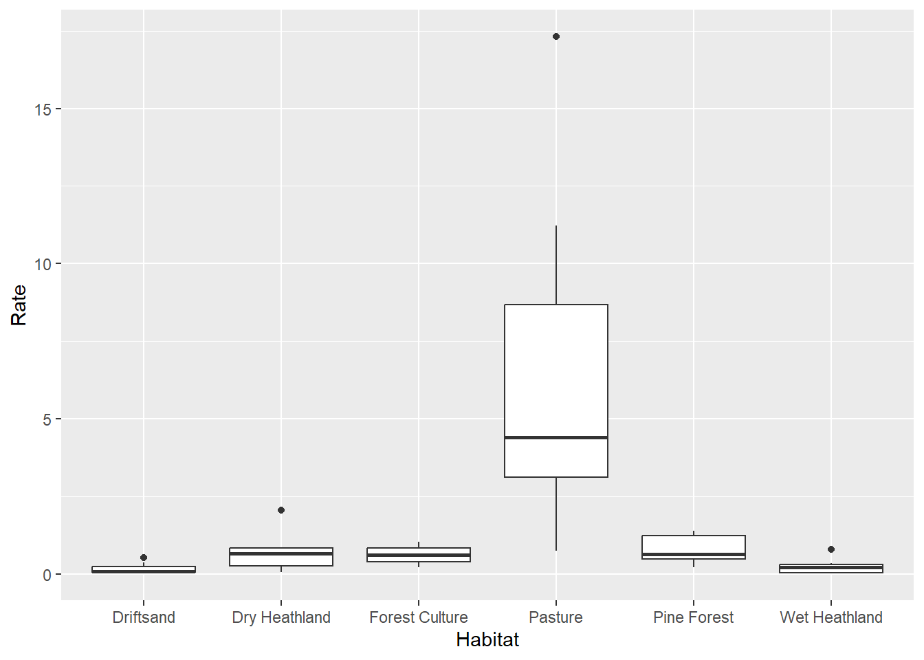
Exercise 3.8b
Create a new variable: the total number of deer over the entire year,
per row (here, each row is a unique station). Call the new variable
sumDeer. In the same mutate statement, compute
a new variable called diffDeer that is the difference
between the newly created column sumDeer and the existing
column Total. Compute the sum of the absolute values of
diffDeer to check the agreement between
diffDeer and Total: are they the same?
As always, there are different ways to do the same thing. Here, the
function rowSums may be helpful in combination with
select and mutate. To get absolute values, see
the abs function.
deer <- mutate(deer,
               sumDeer = rowSums(select(deer, Jan:Dec)),
               diffDeer = sumDeer - Total)
deer
## # A tibble: 48 × 20
## Station_ID Habitat Restricted Jan Feb Mar Apr May Jun Jul Aug Sep Oct Nov Dec Total Effort_d Rate sumDeer diffDeer
## <chr> <chr> <dbl> <dbl> <dbl> <dbl> <dbl> <dbl> <dbl> <dbl> <dbl> <dbl> <dbl> <dbl> <dbl> <dbl> <dbl> <dbl> <dbl> <dbl>
## 1 H1R0-01 Driftsand 0 0 0 7 3 0 0 0 1 2 15 0 1 29 362 0.0801 29 0
## 2 H1R0-02 Driftsand 0 0 0 0 4 5 0 3 2 0 0 4 1 19 363 0.0523 19 0
## 3 H1R0-03 Driftsand 0 0 4 0 0 0 0 0 2 4 0 4 0 14 225 0.0622 14 0
## 4 H1R0-04 Driftsand 0 0 1 0 1 1 0 0 0 19 3 2 1 28 361 0.0776 28 0
## 5 H1R1-01 Driftsand 1 2 0 10 63 4 11 19 3 5 4 9 3 133 360 0.369 133 0
## 6 H1R1-02 Driftsand 1 0 1 12 37 6 46 27 7 13 14 1 0 164 313 0.524 164 0
## 7 H1R1-03 Driftsand 1 0 1 5 3 12 0 0 1 0 5 27 5 59 327 0.180 59 0
## 8 H1R1-04 Driftsand 1 0 11 0 8 1 0 0 0 0 3 2 1 26 358 0.0726 26 0
## 9 H2R0-01-V04 Wet Heathland 0 0 0 0 0 0 0 0 0 0 0 0 2 2 294 0.00680 2 0
## 10 H2R0-02-V12 Wet Heathland 0 5 1 0 0 3 5 7 2 1 17 23 0 64 363 0.176 64 0
## # ℹ 38 more rows# Check sum of absolute differences
sum(abs(deer$diffDeer))## [1] 0The sum of absolute differences is 0, thus the newly created column
sumDeer is the same as Total! Note that we
could also have used the identical function, but this could
still return FALSE when the sum of absolute differences is
0, e.g. when Total is stored as an integer,
whereas sumDeer is of class numeric (also called
double, real or floating point numbers).
Therefore, the dplyr package also has a function near,
which offers a safe way of comparing if two vectors of floating point
numbers are (pairwise) equal, here combined with the all
function to check whether all pairwise comparisons evaluate to
TRUE:
all(near(deer$Total, deer$sumDeer))## [1] TRUE9 Renaming columns
We have now covered the 6 main functions/verbs from the dplyr
package, yet these are not the only functions that the dplyr package
provides: for example the distinct function is useful for
selecting only unique/distinct rows from a data.frame, the
drop_na for removing rows from a tibble with
NA values (either in the entire row or in selected
columns), the rename function changes the names of
individual variables using new_name = old_name syntax, and
the functions first, last and nth
select, respectively, the first, last and nth
records from the data (groups).
Exercise 3.9a
Rename the column “Station_ID” to the new name “Station”. deer <- rename(deer, Station = Station_ID)10 Challenge
Challenge: combining these verbs
In the obs dataset, there is an easy way of subsetting
the data to keep only data from mammal species: to filter the data where
the column “Class” has the value “Mammals”. Produce a ranking of mammals
by the number of observations. Do this by using the functions
filter, group_by, summarise and
arrange in the appropriate way and order. Plot the result
in a horizontal bar chart. Tip: use geom_col instead of
geom_bar: see the help file of the geom_bar
function why. Moreover, you can add a title to your plot using the
function ggtitle.
As you will have seen in the previous exercise: even when your input
data is ordered by the values of some of the columns (in this case:
decreasing total number n), then ggplot will still plot the
order of the categorical variable (here species) differently, as
ggplot by default orders these variables alphabetically.
Using the reorder function in ggplot, you can
have manual control over the ordering of records in these variables. For
example, by using x = reorder(Species, n) inside of the
aes mapping in ggplot, you can plot the column
“Species”, yet along increasing values of column “n” on the x-axis!
Alternatively, using x = reorder(Species, -n) (note that
only the minus sign is different), plots “Species” on the x-axis along
decreasing values in column “n”.
# Rank the mammals by number of observation
obs1 <- filter(obs, Class == "Mammals") # 21,941 mammal observations remain
obs2 <- group_by(obs1, Species)   # grouped into 11 mammal species
obs3 <- summarise(obs2, n = n())
obs4 <- arrange(obs3, desc(n))  # Red deer is the most commonly observed
obs5 <- filter(obs4, n >= 100)
obs5
## # A tibble: 7 × 2
## Species n
## <chr> <int>
## 1 Cervus elaphus 12020
## 2 Ovis ammon musimon 3661
## 3 Sus scrofa 2947
## 4 Capreolus capreolus 2733
## 5 Oryctolagus cuniculus 244
## 6 Lepus europaeus 155
## 7 Vulpes vulpes 119# Plot
ggplot(data = obs5,
mapping = aes(x = Species, y = n, fill = n)) +
geom_col() +
coord_flip() +
ggtitle("Species rank")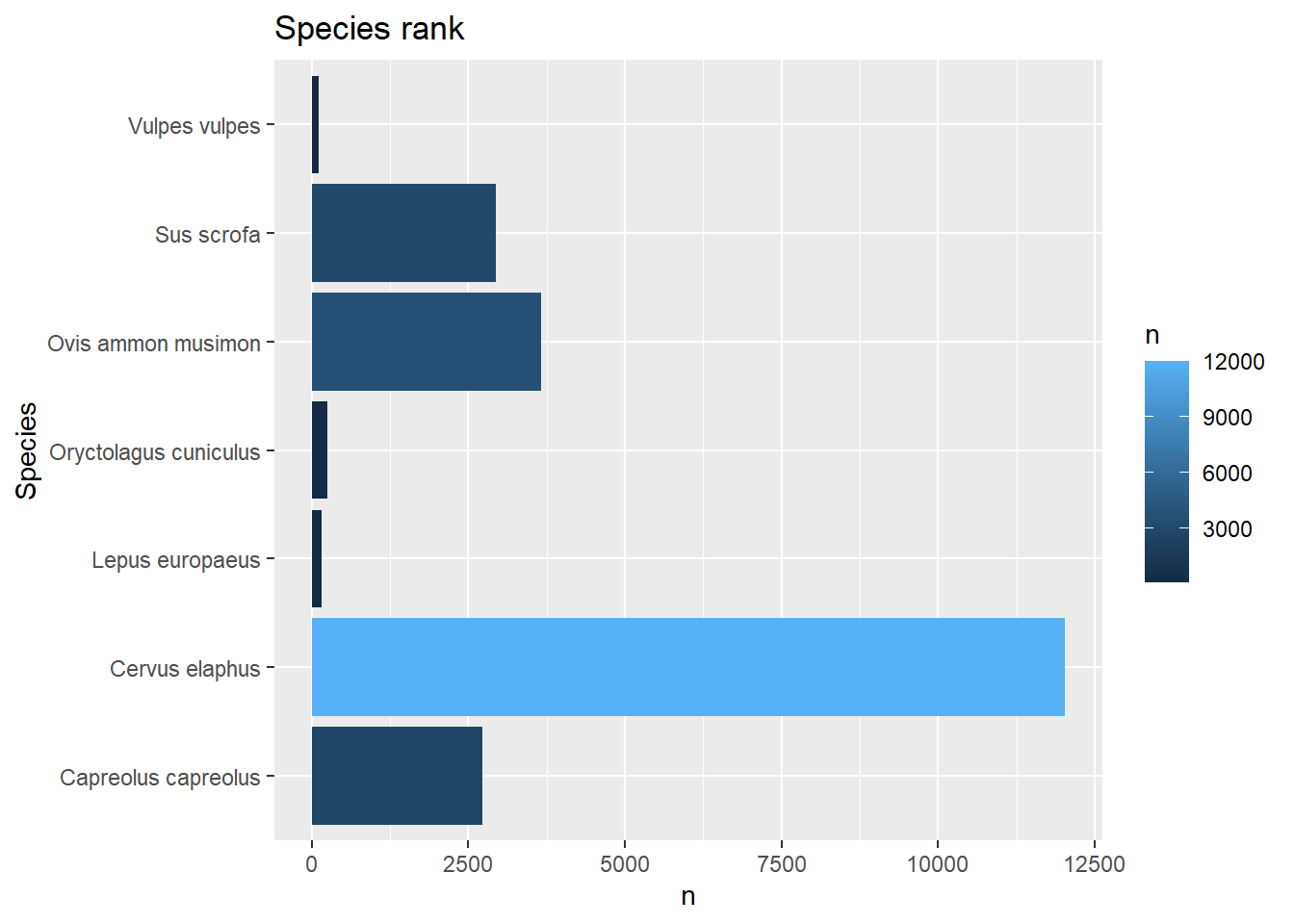
# Plot reordered
ggplot(data = obs5,
       mapping = aes(x = reorder(Species, n), y = n, fill = n)) +
  geom_col() +
  coord_flip() +
  ggtitle("Species rank") +
  labs(x = "Species", y= "Number of observations") +
  scale_y_log10() + #use a log10 scale for n
  annotation_logticks(sides="b") #show log scale ticks
11 Submit your last plot
Submit your script file as well as a plot: either your last created plot, or a plot that best captures your solution to the challenge. Submit the files on Brightspace via Assessment > Assignments > Skills day 3.
Note that your submission will not be graded or evaluated. It is used only to facilitate interaction and to get insight into progress.
12 Recap
Today, we’ve explored the main functions from the dplyr package to transform data. Tomorrow, we are going use a pipe operator to efficiently chain these functions in a pipeline.
An R script of today’s exercises can be downloaded here
13 Further reading
Further reading