Tidymodels
Today’s goal: to get acquainted with using the tidymodels packages for model training and model evaluation.
- R4DS: no R4DS chapters
- Tidy Modeling with R
- a gentle introduction to tidymodels
- modelling with tidymodels and parsnip
tidymodels, consisting of: rsample, recipes, parsnip, yardstick, tune and other packages.
initial_split, training, testing, linear_reg, set_engine, fit, predict, metrics, recipe, step_log, step_center, step_scale, step_normalize, prep, bake
No cheatsheets available yet
1 Introduction
We hope that by now the tidyverse package has given you some fluency
in data transformation and visualization, as well as some tools to model
data (as we saw yesterday in the tutorial). But do you recall that in
the introduction lecture we resembled R to the wild west, as
anything goes? Also in data modelling/machine learning, R contains an
expansive universe of packages and functions, each with their own
interfaces (function names, arguments names) and types of objects
returned. For example, to run a simple linear regression model in R, you
can choose to use the function lm, but also
glm, glmnet or other functions and packages
(and for other machine learning algorithms it is no different: for
example a Random Forest can be run using either
randomForest, ranger or xgboost).
Altogether, this complicates the modelling step in a data science
project.
Developing models can thus benefit from a more unified modelling syntax and a tidy philosophy. This is where the tidymodels package comes in: it provides a tidyverse-friendly unified interface to the modelling part of a data science project: from preprocessing, model training, model prediction to model validation. Tidymodels provides the tools needed to iterate and explore modelling tasks with a tidy philosophy, and shares a common philosophy (and a few libraries) with the tidyverse. The packages in tidymodels do not implement the machine learning algorithms themselves; rather they provide the unified interface to it. In doing so, they make the tasks around model fitting much easier.
Like tidyverse, the package tidymodels is actually a metapackage: when tidymodels is installed or loaded, a set of packages is installed or loaded, including rsample, recipes, parsnip and yardstick. These packages all have their own specific role in the modelling component of data science:
- rsample can be used for different types of data sampling and subsetting (e.g. in train and test sets);
- recipes is a package for data preprocessing: it allows you to record data recipes: the steps that need to be taken in the preprocessing of data;
- parnip is a package that offers a common interface for model training: many algorithms implemented in R have different interfaces and arguments names and parsnip standardizes the interface for fitting models as well as the return values;
- yardstick offers various model performance measures;
- dials and tune can be used for (hyper-)parameter tuning
The gentle introduction to tidymodels places the tidymodels packages as follows in the workflow as shown in the R4DS book and in the lectures:
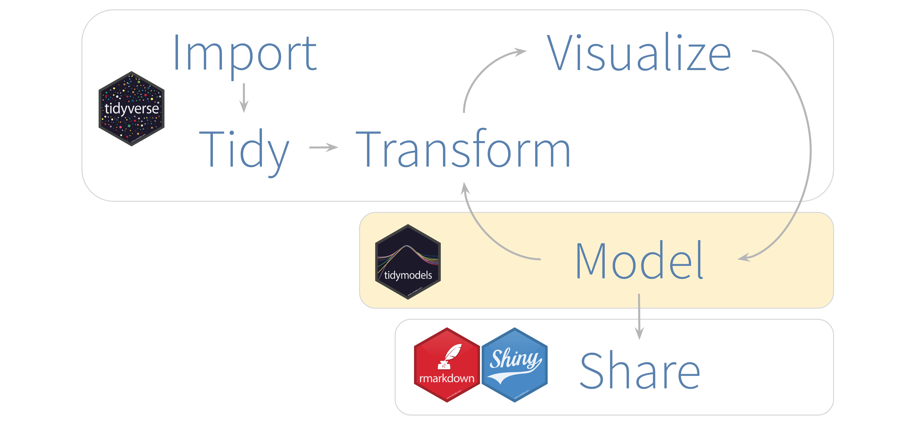
In a way, the model step itself has sub-steps, for which tidymodels thus provides one or several packages:

Tidymodels is still young and in development (most packages still in version 0.x), so at present the amount of documentation is not very abundant, and supported models are not very many yet (but still many good ones are supported!). However, the tidy-philosophy, and also the tidymodels framework has large momentum, so it is evolving to be the central set of packages when it comes to modelling in R.
Some may now be wondering: what about the caret package? Many of the packages in tidymodels contain improved versions of the older, large and famous caret functions, made by the same authors of the tidymodels packages. The caret package does not adhere to a tidy-philosophy, and is a large package that tries to accommodate everything in 1 place. The tidymodels packages, however, have split up the various tasks in smaller functions in separate packages, all based on the same tidy principles.
2 Forest structure data
We will explore the tidymodels functions using the dataset that we used in tutorial 2: the dataset of aboveground biomass in forests across Europe and Asia (Schepaschenko et al. 2017).
dat.
library(tidyverse)
library(tidymodels)
dat <- read_csv("data/raw/forest/Forest biomass data.csv")
In tutorial 2, we’ve subsetted the data to aspen trees only, and
plotted the aboveground biomass (variable AGB) as function of
stand age (variable Stand_age), adding a straight line
(geom_smooth with method = "lm") through the
data:
dat_aspen <- subset(dat, Species == "aspen")
ggplot(data = dat_aspen) +
  geom_point(mapping = aes(x = Precip_annual, y = AGB, size = Stand_age)) +
  geom_smooth(mapping = aes(x = Precip_annual, y = AGB), method = "lm", se = FALSE)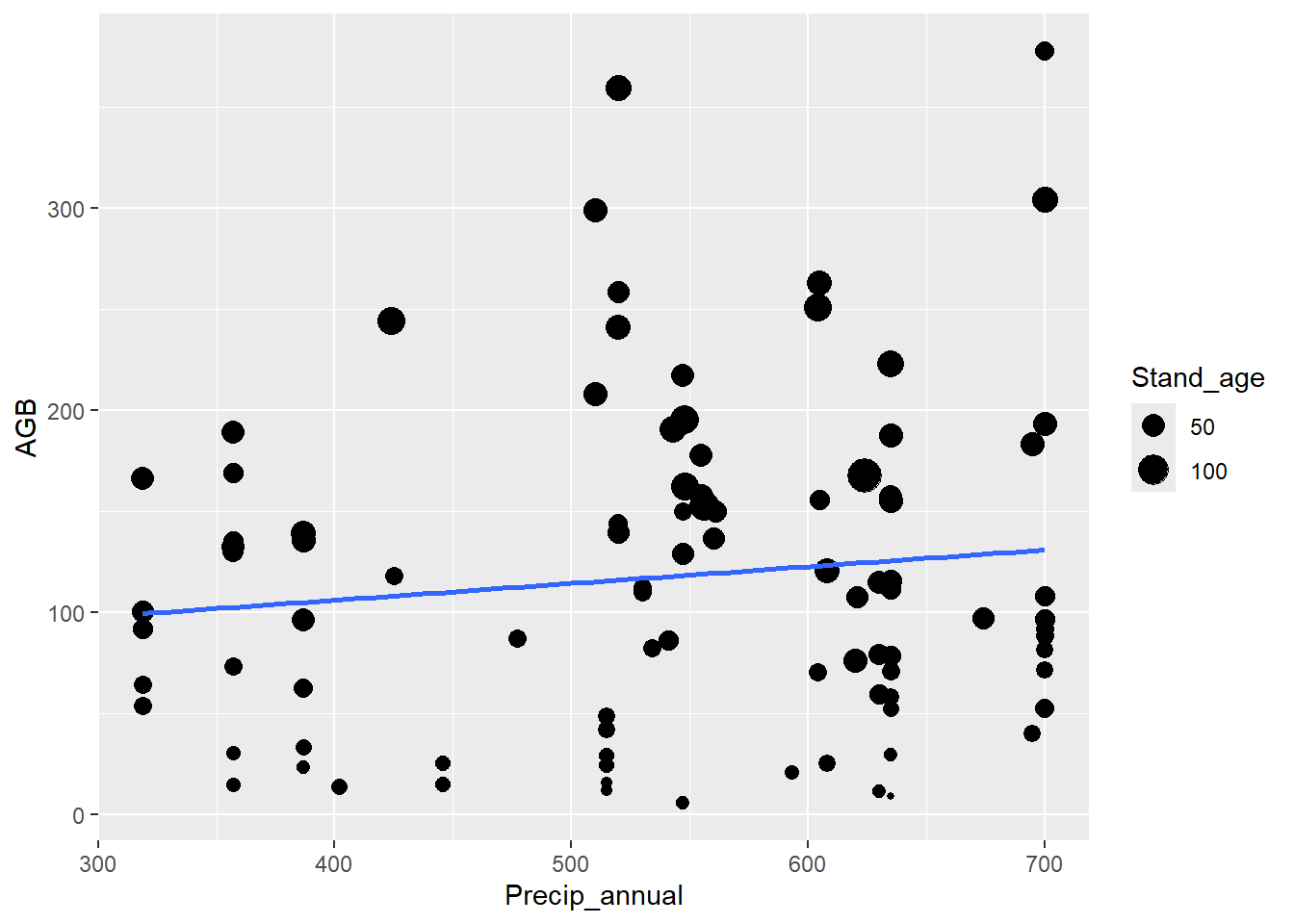
Below we will be using this subset of data for aspen to explore some of the functions of tidymodels.
Since the focus today is on the modelling workflow, we are keeping the steps of data exploration and preparation to a bare minimum, and only use a very simple model: a linear regression as in the figure created above. Some steps of the modelling workflow using the tidymodels toolset we will not explore yet today, but rather next week.
3 Data splits
As discussed in the lectures, for predictive modelling we have to
train the model on a separate part of the data and evaluate the model’s
predictive performance on the withheld data (which was thus not used
during model training). The rsample package provides several
functions to automate such data splits. For example, the function
initial_split can be used to apply the most basic
train/test set splitting: randomising the part allocated to each of
these sets. By default, 75% of the data is allocated to the training
dataset and the remainder to the test dataset, but this can be manually
using the prop function argument (which needs a proportion,
thus value between 0 and 1, and not a percentage). The object returned
by the function initial_split is not a tibble: it is an
object of class rsplit, which holds all data but also the
information on how the records are allocated to the train and test data
splits.
dat_aspen data as
created above, and call it dat_split. Allocate 60% of the
records to the training dataset. Have a look at the output of the
created object dat_split: what do you see? Check the
structure of the object dat_split using the functions
names and glimpse. dat_split <- initial_split(dat_aspen, prop = 0.6)
dat_split## <Training/Testing/Total>
## <55/38/93>names(dat_split)## [1] "data" "in_id" "out_id" "id"glimpse(dat_split)## List of 4
## $ data : tibble [93 × 15] (S3: tbl_df/tbl/data.frame)
## ..$ Plot_ID : num [1:93] 24 439 440 963 1810 ...
## ..$ Tree_species : chr [1:93] "Populus tremula" "Populus tremula" "Populus tremula" "Populus tremula" ...
## ..$ Species_code : chr [1:93] "potr" "potr" "potr" "potr" ...
## ..$ Species : chr [1:93] "aspen" "aspen" "aspen" "aspen" ...
## ..$ Origin : chr [1:93] "Natural" "Natural" "Natural" "Natural" ...
## ..$ Site_index : num [1:93] 8 5 5 6 7 7 6 5 5 5 ...
## ..$ Stand_age : num [1:93] 30 55 51 26 9 19 32 38 49 57 ...
## ..$ Height : num [1:93] 9 23 22.2 14 4.5 10.2 16.5 21.2 27.2 27.1 ...
## ..$ DBH : num [1:93] 10 20 19 12.8 1.9 6.8 10.5 17.2 22.5 29.5 ...
## ..$ Tree_density : num [1:93] 2331 1458 1004 4999 15560 ...
## ..$ Growing_stock: num [1:93] 96 430 292 248 14 ...
## ..$ AGB : num [1:93] 52.4 299.1 208 118 11.4 ...
## ..$ Temp_annual : num [1:93] 0.7875 -0.5458 -0.5458 0.0667 5.3625 ...
## ..$ Precip_annual: num [1:93] 700 510 510 425 630 608 630 630 630 608 ...
## ..$ CEC_Soil : num [1:93] 41 64 64 38 25 32 25 25 25 32 ...
## $ in_id : int [1:55] 78 27 33 34 59 80 39 64 7 65 ...
## $ out_id: logi NA
## $ id : tibble [1 × 1] (S3: tbl_df/tbl/data.frame)
## ..$ id: chr "Resample1"
## - attr(*, "class")= chr [1:3] "initial_split" "mc_split" "rsplit"
## - attr(*, "prop")= num 0.6
## - attr(*, "breaks")= num 4
## - attr(*, "pool")= num 0.1To retrieve the data allocated to the training set, use the
training function. Idem, use testing for
retrieving the data allocated to the testing set.
dat_split %>%
  training() %>%
  glimpse()
## Rows: 55
## Columns: 15
## $ Plot_ID <dbl> 9126, 3326, 3333, 3334, 5779, 9128, 3339, 5786, 1812, 5787, 9156, 1823, 1835, 5782, 3332, 9115, 3327, 3329, 3344, 1811, 9137, 1822, 3337, 33…
## $ Tree_species <chr> "Populus tremula", "Populus tremula", "Populus tremula", "Populus tremula", "Populus tremula", "Populus tremula", "Populus tremula", "Populu…
## $ Species_code <chr> "potr", "potr", "potr", "potr", "potr", "potr", "potr", "potr", "potr", "potr", "potr", "potr", "potr", "potr", "potr", "potr", "potr", "pot…
## $ Species <chr> "aspen", "aspen", "aspen", "aspen", "aspen", "aspen", "aspen", "aspen", "aspen", "aspen", "aspen", "aspen", "aspen", "aspen", "aspen", "aspe…
## $ Origin <chr> "Natural", "Natural", "Natural", "Natural", "Natural", "Natural", "Natural", "Natural", "Natural", "Natural", "Natural", "Natural", "Natural…
## $ Site_index <dbl> 7, 7, 5, 6, 6, 4, 10, 7, 6, 7, 5, 6, 6, 6, 5, 7, 6, 6, 7, 7, 6, 6, 7, 7, 6, 5, 6, 7, 9, 6, 7, 7, 6, 6, 6, 5, 5, 5, 5, 7, 5, 8, 5, 5, 5, 5, 6…
## $ Stand_age <dbl> 10, 19, 28, 46, 48, 50, 80, 23, 32, 26, 42, 33, 45, 49, 16, 35, 6, 19, 26, 19, 45, 24, 15, 31, 75, 38, 25, 26, 45, 54, 12, 55, 42, 13, 58, 5…
## $ Height <dbl> 4.9, 10.2, 16.6, 18.1, 23.0, 28.0, 10.0, 10.3, 16.5, 12.5, 21.3, 19.0, 20.0, 21.8, 7.2, 16.0, 3.8, 12.5, 11.4, 10.2, 16.0, 13.7, 8.5, 12.9, …
## $ DBH <dbl> 2.2, 7.2, 12.6, 15.2, 20.8, 25.2, 14.5, 7.5, 10.5, 12.5, 19.1, 11.4, 17.0, 20.1, 4.5, 14.0, 2.5, 8.7, 8.1, 6.8, 13.0, 8.5, 4.4, 9.9, 27.0, 1…
## $ Tree_density <dbl> 11630, 4320, 1412, 1355, 1061, 648, 2778, 4074, 2960, 1431, 1428, 2600, 1160, 961, 9267, 1387, 25723, 3360, 7770, 3020, 1675, 3800, 8100, 68…
## $ Growing_stock <dbl> 12.1, 97.5, 128.0, 188.0, 417.0, 500.0, 511.0, 95.0, 161.0, 113.0, 386.0, 234.0, 220.0, 284.0, 56.0, 172.0, 28.3, 109.0, 176.0, 60.0, 270.0,…
## $ AGB <dbl> 5.7000, 41.9300, 62.4100, 96.3800, 189.3000, 217.0000, 244.3500, 54.0900, 59.6500, 64.2500, 258.5800, 111.4280, 107.7000, 132.5500, 33.4300,…
## $ Temp_annual <dbl> 6.2375000, -0.7291666, 1.1875000, 1.1875000, 1.3125001, 6.2375000, -1.4500000, 2.1625000, 5.3625000, 2.1625000, -1.1333333, 3.6583333, 4.699…
## $ Precip_annual <dbl> 547, 515, 387, 387, 357, 547, 424, 319, 630, 319, 520, 635, 621, 357, 387, 635, 515, 515, 700, 608, 560, 635, 446, 700, 635, 630, 477, 530, …
## $ CEC_Soil <dbl> 29.5, 52.0, 33.0, 33.0, 31.5, 29.5, 38.5, 29.0, 25.0, 29.0, 53.0, 41.0, 33.0, 31.5, 33.0, 25.5, 52.0, 52.0, 41.0, 32.0, 31.0, 41.0, 46.5, 41…dat_train and dat_test,
reespectively. dat_train <- dat_split %>% training()
dat_test <- dat_split %>% testing()Avoid data leakage! Data leakage, according to quora, refers to an error made by the creator of a machine learning model in which accidentally information is shared between the training and test data sets. In general, by dividing a set of data into training and test sets, the goal is to ensure that no data is shared between the two.
The rsample package contains more powerful methods for splitting data in training and testing sets! For example:
- in the function
initial_splityou can use the argumentstratato conduct stratified sampling; - the function
initial_time_splittakes the firstpropsamples for training, instead of a random selection; - the function
vfold_cvrandomly splits the data into V groups of roughly equal size (called folds), thus useful for V-fold cross validation; loo_cvcan be used for leave-one-out cross validation.group_vfold_cvperforms V-fold cross-validation based on some grouping variable: a common use of this kind of resampling is when you have repeated measures of the same subject.
We will see some of these other forms of data splits later, but for now we stick to the random allocation of all data in train and test sets.
4 Data preprocessing
The recipes package uses a cooking metaphor to handle all the data preprocessing, like missing values imputation, removing predictors, centering and scaling, converting factor levels into dummy variables, and more. Using the recipes package, we can store all the preprocessing steps in a single object, so that it can later be applied to new (raw) input data, resulting in a preprocessed version of the new raw data. In that way, using a data recipe we can preprocess raw data that after preprocessing is ready for use in a machine learning algorithm.
The recipes package contains many possible transformations that you
can use to preprocess the data, all functions have the form
step_*(). Using these steps, you can define a
recipe for the transformations that you want to apply to the
data.
The recipe is generally specified with a dataset: this data is used
to estimate some of the values of the recipe steps, such as the number
of dummy variables created. However, the recipe isn’t “trained” yet.
Training (or preparing) the data recipe here means
that the necessary values for feature engineering will be calculated and
stored in the recipe. For example, for feature centering
(i.e. removing the mean value from the feature values), we need
to know the mean value of the feature. Or, for feature scaling
(i.e. converting the scale of the feature such that the standard
deviation is 1), we need to know the standard deviation of the feature.
Centering and scaling can be done with step_center and
step_scale, respectively. Note that feature
standardization refers to both centering and scaling, thus
after standardization the mean of that feature = 0 and the standard
deviation = 1 (generally this is written as “we standardize the feature
to zero-mean and unit-variance”).
To train a recipe, we can use the prep
function: but note that training the data recipe should only be done on
the training dataset, and not the test dataset! This
eliminates a possible source of data leakage.
Recall from above the problem of data leakage (e.g: transferring information from the train set into the test set): a data recipe should be prepped with the training data only!
Finally, to continue with the cooking metaphor, you can bake the recipe to apply all preprocessing to the data sets: indeed this can be either the training dataset or the testing dataset!
To practice, let’s prepare a data recipe that formulates a model structure, and performs some transformations (centering and scaling) on the predictor variable.
dat_train,
that specifies that the response is AGB and the predictor
variable is Stand_age, where the predictor variable is (1)
transformed via a log-transformation, (2) centered (i.e. the mean of the
variable is subtracted from all values), and (3) scaled (i.e. all values
are divided by the standard deviation, so that the scale of the data is
in units variance). Assign the data recipe to an object called
lmrecipe, and look at the object by printing it to the
console. lmrecipe <- dat_train %>%
recipe(AGB ~ 1 + Stand_age) %>%
step_log(Stand_age) %>%
step_center(Stand_age) %>%
step_scale(Stand_age)
lmrecipelmrecipe and have a look at the output. lmrecipe <- lmrecipe %>%
prep(training = dat_train)
lmrecipeYou now see that some more information is added to the data recipe:
it not only states that some columns are transformed (log, centering,
scaling), but also where the information for the transformations is
taken from: here from [trained].
dat_train and
dat_test), and store the resultant preprocessed dataset as
dat_train_prepped and dat_test_prepped,
respectively (to clearly indicate the type of dataset you’re working
with: train or test, and preprocessed or
not). Have a look at both datasets. dat_train_prepped <- lmrecipe %>%
bake(dat_train)
dat_test_prepped <- lmrecipe %>%
bake(dat_test)
dat_train_prepped## # A tibble: 55 × 2
## Stand_age AGB
## <dbl> <dbl>
## 1 -1.69 5.7
## 2 -0.745 41.9
## 3 -0.176 62.4
## 4 0.553 96.4
## 5 0.616 189.
## 6 0.676 217
## 7 1.37 244.
## 8 -0.464 54.1
## 9 0.0205 59.6
## 10 -0.284 64.2
## # ℹ 45 more rowsdat_test_prepped## # A tibble: 38 × 2
## Stand_age AGB
## <dbl> <dbl>
## 1 -0.0743 52.4
## 2 0.816 299.
## 3 -0.284 118.
## 4 -1.84 11.4
## 5 0.646 115.
## 6 -1.84 29.8
## 7 -0.997 52.4
## 8 -0.598 58.4
## 9 0.553 157.
## 10 0.152 156.
## # ℹ 28 more rowsNow, in each dataset you see only 2 columns: where Stand_age
is transformed using the above data recipe! Isn’t this cool?! Once
you’ve set up a data recipe, you can bake your raw data in 1
statement to a format that is suitable input for machine learning
algorithms. Here, we’ve only done some very small data transformations
(log, center and scale), but the list of step_ functions is
very long: for example we can convert factor columns into
dummy columns (columns with value 0 or 1, so that each level in
the factor gets a unique combination of zeros and ones).
5 Model training
As introduced above, the tidymodels package, and here in particular the parsnip package, aims at providing a unified interface to the various machine leaning algorithms offered in R (currently a selection, but this is increasing). So instead of different functions (possibly from different packages) that implements a similar algorithm (e.g. Random Forest, linear regression or Support Vector Machine), parsnip provides a single interface (i.e. function with standardized argument names) for each of the classes of models. See this list of models currently implemented in parsnip.
For example, to execute a linear regression model using tidymodels,
we can thus use the function linear_reg.
linear_reg function from the
parsnip package. ?parsnip::linear_regWe see that the linear_reg function has input arguments:
mode, engine, penalty, and
mixture. The mode can be set to “regression”
(default) or “classification”, thus specifying the task that the
algorithm should perform. The engine specifies the
computational engine that should be used for fitting: these are the
different implementations of an algorithm (here linear model) that can
be used to fit the model to data. The arguments penalty and
mixture can be used to specify the type and amount of
regularization in the model (e.g. the regularization parameter for lasso
and ridge regression).
Although you can thus specify the engine when defining the model
(here e.g. via the linear_reg function), below we will
specify the engine separately, which allows for more options,
e.g. setting engine arguments separately.
What the function linear_reg allows us to do is to
specify the model before we are going to fit it to
data.
linear_reg function to specify a linear regression
model. linear_reg(mode = "regression")## Linear Regression Model Specification (regression)
##
## Computational engine: lmBefore we can fit the model, we have to specify which
engine is going to do the fitting for us. The function
set_engine is used to specify which package or system will
be used to fit the model, along with any arguments specific to that
software. See in the
list
of models that for a linear regression (linear_reg) we
can for example choose the engine lm, which will use the
lm function in base R to estimate the specified linear
regression for us. Like linear_reg specifies the type of
model we want to fit to the data, set_engine specifies the
engine that is doing the actual estimation. However, it is not yet going
to conduct the estimation, i.e. it is not yet fitting the model
to the data. For that, we need to call the fit
function.
set_engine and fit
functions ?set_engine
?fitDo you notice that both functions start with the argument
object? This is convenient (and deliberately chosen),
because we can now combine these functions in a pipe (like in
tidyverse where the first argument in most functions is
.data so that we can combine them in a pipe). In the
fit function, we can specify the linear regression model
just as we would do using the lm model (recall that a
linear regression is carried out using the lm function
using the syntax lm(y ~ x, data = dat, where y
is the response variable, x the predictor variable, and
dat the data).
dat_train_prepped, where the column AGB is the
response variable, the column Stand_age the predictor
variable). Set the engine used for fitting to lm.
Assign the fitted model to the object with name dat_lm.
Check the output by printing it to the console dat_lm <- linear_reg(mode = "regression") %>%
set_engine("lm") %>%
fit(AGB ~ 1 + Stand_age,
data = dat_train_prepped)
dat_lm## parsnip model object
##
##
## Call:
## stats::lm(formula = AGB ~ 1 + Stand_age, data = data)
##
## Coefficients:
## (Intercept) Stand_age
## 124.70 61.48Do you notice that you now have fitted a “parnip model object”? This is very convenient: not only the interface to the engine that is fitting the specified model is unified, also the output returned is always in a unified format. Parsnip, and thus tidymodels, thus provides a unified way of fitting models to data in R!
Above we used the function linear_reg to
specify a linear regression model. To specify a linear model
that can do binary classification, i.e. logistic regression, use
logistic_reg. The default engine of
linear_reg is lm, whereas that of
logistic_reg is glm, but this can be changed
via the set_engine function.
In contrast to linear models, some algorithms can be applied to both
types of problems: setting the mode to either “regression”
or “classification” in de specification of that model allows you to
specify which type of problem you want the algorithm to model. These
other algorithms can include:
- Random forest: specify via
rand_forest, where the default engine is “ranger”; - Gradient boosted tree: specify via
boost_tree, where the default engine is “xgboost”; - Support Vector Machine (SVM): for a linear SVM use
svm_linear(with default engine “LiblineaR”), whereas for a kernel SVM (or radial basis function SVM) usesvm_rbf(with default engine “kernlab”); - Artificial Neural Network: use
mlp(a multilayer perceptron model a.k.a. a single layer, feed-forward neural network, with default engine “nnet”).
Note that the common hyperparameters per algorithm type can be
specified within the model specification function (e.g. for Random
forest the rand_forest function), whereas
engine-specific hyperparameters can be specified in the
set_engine function!
For the full list op parsnip interface options, including engines and engine-specific hyperparameters, see the list of models currently implemented in parsnip.
6 Model predictions
Using the predict function, we can predict a fitted
model on (new) data. In tidymodels, also the data that is returned by
the predict function is standardized: it returns a
tibble with the column .pred containing the model
predictions. It can be merged with the data simply using the
bind_cols function.
dat_test_prepped) dat_lm %>%
predict(dat_test_prepped)## # A tibble: 38 × 1
## .pred
## <dbl>
## 1 120.
## 2 175.
## 3 107.
## 4 11.5
## 5 164.
## 6 11.5
## 7 63.4
## 8 87.9
## 9 159.
## 10 134.
## # ℹ 28 more rowsdat_test data and assign the result to a new
object called dat_testfit dat_testfit <- dat_lm %>%
predict(dat_test_prepped) %>%
bind_cols(dat_test)
dat_testfit## # A tibble: 38 × 16
## .pred Plot_ID Tree_species Species_code Species Origin Site_index Stand_age Height DBH Tree_density Growing_stock AGB Temp_annual Precip_annual CEC_Soil
## <dbl> <dbl> <chr> <chr> <chr> <chr> <dbl> <dbl> <dbl> <dbl> <dbl> <dbl> <dbl> <dbl> <dbl> <dbl>
## 1 120. 24 Populus tremula potr aspen Natural 8 30 9 10 2331 96 52.4 0.788 700 41
## 2 175. 439 Populus tremula potr aspen Natural 5 55 23 20 1458 430. 299. -0.546 510 64
## 3 107. 963 Populus tremula potr aspen Natural 6 26 14 12.8 4999 248 118. 0.0667 425 38
## 4 11.5 1810 Populus tremula potr aspen Natural 7 9 4.5 1.9 15560 14 11.4 5.36 630 25
## 5 164. 1814 Populus tremula potr aspen Natural 5 49 27.2 22.5 800 358 115. 5.36 630 25
## 6 11.5 1817 Populus tremula potr aspen Natural 6 9 6.4 3.5 18580 67 29.8 3.66 635 41
## 7 63.4 1818 Populus tremula potr aspen Natural 7 16 8.3 4.9 10080 92.9 52.4 3.66 635 41
## 8 87.9 1820 Populus tremula potr aspen Natural 7 21 10.7 6.5 6700 127 58.4 3.66 635 41
## 9 159. 1826 Populus tremula potr aspen Natural 5 46 22.9 20.6 880 316 157. 3.66 635 41
## 10 134. 2433 Populus tremula potr aspen Natural 6 35 16 12 3018 246 156. 2.51 605 35
## # ℹ 28 more rowsdat_testfit %>%
ggplot(mapping = aes(x = Stand_age, y = .pred)) +
geom_line(col = "red") +
geom_point(mapping = aes(y = AGB))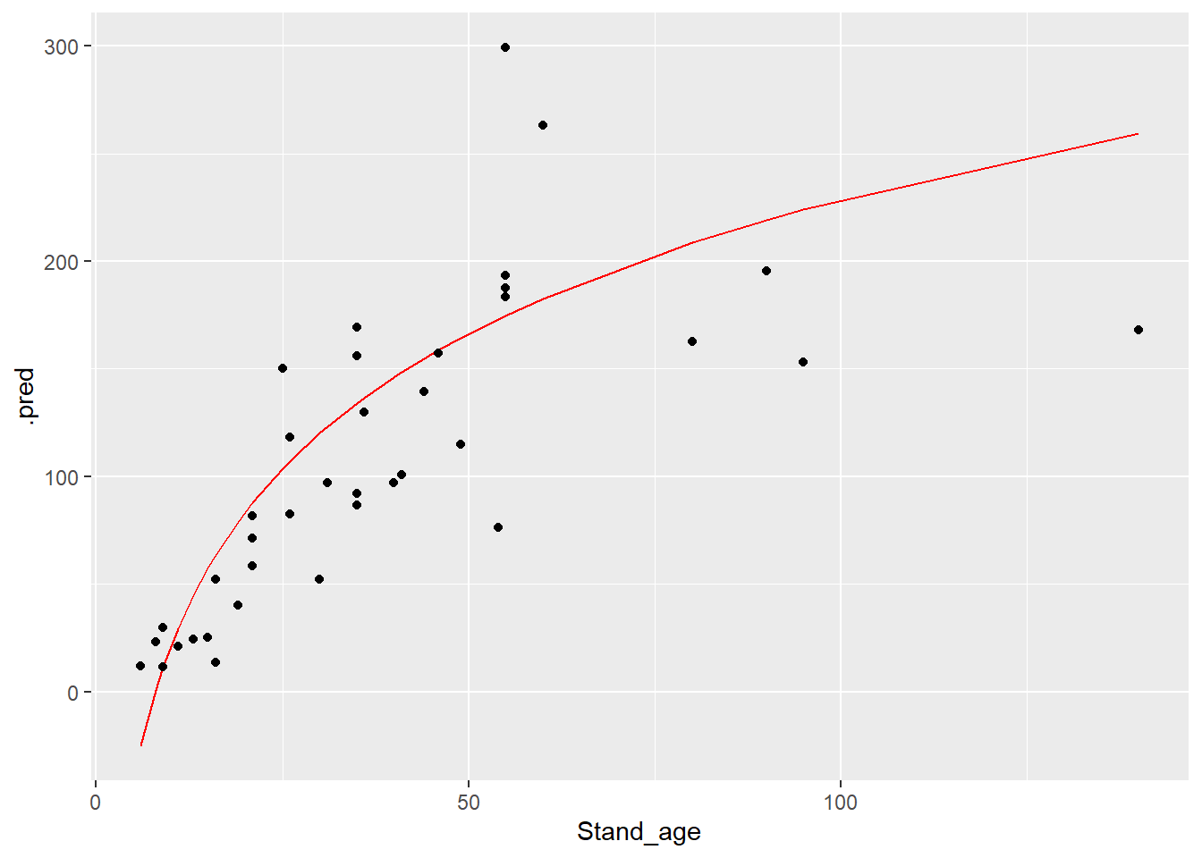
7 Model validation
The yardstick package offers the function
metrics which returns several measures of model
performance.
metrics function, and pay
attention to the first function arguments. ?metricsNotice the first 3 function arguments: data,
truth, and estimate, where data
should be a data.frame/tibble, and truth and
estimate the names of the columns containing the actual and
predicted data in data. Which metrics are returned is
dependent on the type of task performed (e.g. classification
vs. regression), and the type of algorithm used.
dat_testfit %>%
  metrics(truth = AGB, estimate = .pred)
## # A tibble: 3 × 3
## .metric .estimator .estimate
## <chr> <chr> <dbl>
## 1 rmse standard 45.4
## 2 rsq standard 0.634
## 3 mae standard 35.78 Challenge
With the preprocessed data dat_train_prepped and
dat_test_prepped, model the relationship between
AGB (as reponse) and Stand_age (as predictor) using
different algorithms: linear regression, random forest regression, and
kernel SVM regression.
Train the models using the training data. Next week we will be doing hyperparameter tuning, however for now we use some preset hyperparameter values:
- for the random forest, use the default “ranger” engine; set the
hyperparameter
min_nto value 10 and the engine-specific hyperparametermax.depthto value 3; - Tor the kernel SVM, use the default “kernlab” engine, set the
hyperparameter value
costto value 1 andrbf_sigmato value 0.1.
Predict the fitted models to the test dataset, and plot the results in graph: plot both the raw datapoints, as well as the fitted regression lines, and make sure to plot original values for Stand_age, and not the transformed values!
Which of these algorithms model the relationship between stand age and aboveground biomass best?We can fit the different algorithms using the training data as follows:
# Linear regression
fit_lm <- linear_reg(mode = "regression") %>%
  set_engine("lm") %>%
  fit(AGB ~ 1 + Stand_age,
      data = dat_train_prepped)

# Random forest
fit_rf <- rand_forest(mode = "regression",
                      min_n  = 10) %>%
  set_engine("ranger", max.depth = 3) %>%
  fit(AGB ~ 1 + Stand_age,
      data = dat_train_prepped)

# kernel SVM
fit_svm <- svm_rbf(mode = "regression",
                    cost = 1,
                    rbf_sigma = 0.1) %>%
  set_engine("kernlab") %>%
  fit(AGB ~ 1 + Stand_age,
      data = dat_train_prepped)
Then, using the fitted models, we can make predictions on the test dataset:
pred_lm <- fit_lm %>%
  predict(dat_test_prepped)
pred_rf <- fit_rf %>%
  predict(dat_test_prepped)
fit_svm <- fit_svm %>%
  predict(dat_test_prepped)
Then, we can combine the data, convert to a long format, visualize the predictions and compute prediction performance metrics:
# Merge
pred_all <- bind_cols(rename(pred_lm, .pred_lm = .pred),
                      rename(pred_rf, .pred_rf = .pred),
                      rename(fit_svm, .pred_svm = .pred),
                      dat_test)
pred_all
## # A tibble: 38 × 18
## .pred_lm .pred_rf .pred_svm Plot_ID Tree_species Species_code Species Origin Site_index Stand_age Height DBH Tree_density Growing_stock AGB Temp_annual
## <dbl> <dbl> <dbl> <dbl> <chr> <chr> <chr> <chr> <dbl> <dbl> <dbl> <dbl> <dbl> <dbl> <dbl> <dbl>
## 1 120. 219. 98.5 24 Populus tremula potr aspen Natural 8 30 9 10 2331 96 52.4 0.788
## 2 175. 152. 168. 439 Populus tremula potr aspen Natural 5 55 23 20 1458 430. 299. -0.546
## 3 107. 84.1 82.9 963 Populus tremula potr aspen Natural 6 26 14 12.8 4999 248 118. 0.0667
## 4 11.5 19.5 11.3 1810 Populus tremula potr aspen Natural 7 9 4.5 1.9 15560 14 11.4 5.36
## 5 164. 151. 155. 1814 Populus tremula potr aspen Natural 5 49 27.2 22.5 800 358 115. 5.36
## 6 11.5 19.5 11.3 1817 Populus tremula potr aspen Natural 6 9 6.4 3.5 18580 67 29.8 3.66
## 7 63.4 29.4 39.1 1818 Populus tremula potr aspen Natural 7 16 8.3 4.9 10080 92.9 52.4 3.66
## 8 87.9 45.0 61.6 1820 Populus tremula potr aspen Natural 7 21 10.7 6.5 6700 127 58.4 3.66
## 9 159. 145. 148. 1826 Populus tremula potr aspen Natural 5 46 22.9 20.6 880 316 157. 3.66
## 10 134. 124. 116. 2433 Populus tremula potr aspen Natural 6 35 16 12 3018 246 156. 2.51
## # ℹ 28 more rows
## # ℹ 2 more variables: Precip_annual <dbl>, CEC_Soil <dbl># Rearrange and pivot to "long" format
pred_all_long <- pred_all %>%
select(AGB, Stand_age, starts_with(".pred_")) %>%
pivot_longer(starts_with(".pred_"),
names_to = "algorithm",
values_to = "prediction") %>%
mutate(algorithm = str_remove_all(algorithm, pattern = ".pred_") )
pred_all_long## # A tibble: 114 × 4
## AGB Stand_age algorithm prediction
## <dbl> <dbl> <chr> <dbl>
## 1 52.4 30 lm 120.
## 2 52.4 30 rf 219.
## 3 52.4 30 svm 98.5
## 4 299. 55 lm 175.
## 5 299. 55 rf 152.
## 6 299. 55 svm 168.
## 7 118. 26 lm 107.
## 8 118. 26 rf 84.1
## 9 118. 26 svm 82.9
## 10 11.4 9 lm 11.5
## # ℹ 104 more rows# plot
pred_all_long %>%
ggplot(mapping = aes(x = Stand_age)) +
geom_line(mapping = aes(y = prediction, col = algorithm)) +
geom_point(mapping = aes(y = AGB)) +
labs(x = "Stand age (year)",
y = "Aboveground biomass",
col = "Algorithm")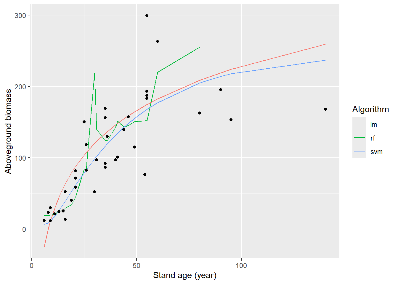
# retrieve metrics
pred_all %>% metrics(truth = AGB, estimate = .pred_lm)
## # A tibble: 3 × 3
## .metric .estimator .estimate
## <chr> <chr> <dbl>
## 1 rmse standard 45.4
## 2 rsq standard 0.634
## 3 mae standard 35.7pred_all %>% metrics(truth = AGB, estimate = .pred_rf)## # A tibble: 3 × 3
## .metric .estimator .estimate
## <chr> <chr> <dbl>
## 1 rmse standard 54.6
## 2 rsq standard 0.523
## 3 mae standard 39.0pred_all %>% metrics(truth = AGB, estimate = .pred_svm)## # A tibble: 3 × 3
## .metric .estimator .estimate
## <chr> <chr> <dbl>
## 1 rmse standard 41.6
## 2 rsq standard 0.662
## 3 mae standard 29.9With the specified hyperparameter values (which may or may not be chosen wisely!), the SVM seems to fit the data best, followed by the linear model and then the random forest:
- the random forest predicts a quite erratic pattern, which may not represent the true general pattern very well!
- the linear model results in a nice smooth line (by design: here not
linear since the model is trained on a transformed stand age (we used
step_log!). However; the predictions from the linear model become negative at very low stand age! This is unrealistic as this is not possible! (we could have chosen to not model ABG as function of log(stand age), but instead log(AGB) as function fo log(stand age), so that the predictions for AGB never can be negative!); - the SVM also fits the data in a nice smooth manner, even predicting only positive values at young stand age!
- the prediction metrics are best; i.e. highest r2 (rsq) and lowest root mean squared error (rmse) and mean absolute error (mae) for the SVM, and worst for the random forest)
9 Submit your last plot
Submit your script file as well as a plot: either your last created plot, or a plot that best captures your solution to the challenge. Submit the files on Brightspace via Assessment > Assignments > Skills day 9.
Note that your submission will not be graded or evaluated. It is used only to facilitate interaction and to get insight into progress.
10 Recap
Today, we’ve entered the tidymodels ecosystem (itself thus a collection of packages akin to tidyverse). Tomorrow, we’ll practice making reproducible reports using RMarkdown with a challenge to build an interactive Shiny app!
An R script of today’s exercises can be downloaded here