Keras is a deep learning API written in Python,
running on top of the machine learning platform TensorFlow. It
was developed with a focus on enabling fast experimentation. Being able
to go from idea to result as fast as possible is key to doing good
research.
Keras is simple (but not simplistic), flexible
(simple workflows should be quick and easy, but you can also write
arbitrarily advanced workflows in a clear way), and powerful,
proving both performance and scalability. For more information about the
underlying Python version of Keras, see
here.
In this tutorial, you will continue with the images that you prepared
in tutorial 14.
Exercise 16.2a
Open RStudio where you have keras3 installed. So if you
installed the RStudio Docker container during the previous exercise of
this assignment, then open your corresponding
RStudio Server.
However, if you managed to install keras3 locally in your own
RStudio environment (including the Python and Tensorflow backend), then
you can keep on working in the same RStudio environment as you did
during the rest of the course.
Note that if you run RStudio Server as a docker container, then this
instance of RStudio only has access to the directory that you assigned
as a volume during the creation of the container. This means that you
can not load or save data from other directories on your PC to this
RStudio Server. Also note that within the docker container this working
directory is called "/home/rstudio/workspace", which you
can check by running getwd() in the console of RStudio
Server. This directory from within the container is actually bound to
the directory on your own system, which you defined during the
installation process. You can check if this went alright by eyeballing
the Files tab in RStudio Server, which should display all the
files that are inside the directory you mounted to the docker container
during installation. So also if you save your script or output in this
"/home/rstudio/workspace" directory (or a subfolder inside
it), then these files will appear in the assigned directory on your own
system.
Now first load the tidyverse, imager and
abind packages. Then, load the data you saved at the end of
tutorial 14: the .rds files train0, train1,
val0, val1 and testgrid (make
sure these are present in the mounted working directory). If you want,
you can also download the .rds files from Brightspace (Image
analyses > Data > Images 1 - prepared), as we saved them in
rendering these pages. To load a rds file, you can use the function
read_rds, see tutorial 1.
The imager package is a convenient package to process your
image data (as we saw in tutorial 14), but Keras expects
our data to look a bit different compared to the cimg
objects. So let’s convert our data now to make it suitable to train,
validate and test CNNs with Keras.
Keras expects one array for all your training input data, one array
for all your validation input data and one array for all your test input
data. In these arrays the first dimension represents the different data
records (so images), the second dimension represents the x-coordinate of
the pixels, the third dimension the y-coordinate of the pixels and the
final dimension the colour channels.
Exercise 16.3a
What should the dimensions be for our training, validation and test
data?
We have 200 training images (the 50 selected “bush” and 50
selected “other” images, plus all of them augmented by mirroring along
the vertical axis), 100 validation images and 5047 (which can
differ a bit in your case) test images. All images are 50
pixels wide by 50 pixels high. Finally all images consist of 3 colour
channels (red, green and blue).
This means that our training input data array should become 200 by 50
by 50 by 3, our validation data 100 by 50 by 50 by 3 and our test data
5047 by 50 by 50 by 3.
Exercise 16.3b
Let’s create the input training, validation and test arrays. For this we
need the abind package to bind arrays together. Start by
taking a look at the help file of the abind function of
this package. Now combine the train1 and
train0 objects (in that order!) together into one array
along the third dimension and call it trainx. Also do the
same for the validation set and convert the test set into an array as
well (call the outputs valx and testx,
respectively). You can do this with only one line of code per dataset if
you use the do.call function again, which in this case
should abind all the elements of the lists together. Check afterwards if
the conversion went allright.
# create training, validation and test arrays
trainx <- do.call(abind, list(c(train1, train0), along = 3))
valx   <- do.call(abind, list(c(val1, val0), along = 3))
testx  <- do.call(abind, list(testgrid, along = 3))

# check dimensions
dim(trainx)
## [1] 50 50 200 3
dim(valx)
## [1] 50 50 100 3
dim(testx)
## [1] 50 50 5047 3
Exercise 16.3c
Something is still not right about our input data. Keras want the
first dimension to be the different data records (i.e. images), yet now
we have it mapped to the third dimension of the array. However, we can
change this easily with a base R function:
# change order array elements
trainx <- aperm(trainx, c(3,1,2,4))
dim(trainx)
## [1] 200 50 50 3
valx <- aperm(valx, c(3,1,2,4))
dim(valx)
## [1] 100 50 50 3
testx <- aperm(testx, c(3,1,2,4))
dim(testx)
## [1] 5047 50 50 3
For the labels (or output data), Keras expects one matrix for the
training data, one matrix for the validation data and one matrix for the
test data. The first dimension of this matrix (the rows) again
represents the different data records (so images) and the second
dimension (columns) represents the different labels. Because we want to
perform binary classification, we need to create two labels and thus two
columns.
Exercise 16.3d
Create these matrices now for the training and validation set (for the
test set we did not create the labels) and call them trainy
and valy. Remember that the first half of the records in
the trainx and valx arrays were the images of
bush and the second half of no-bush. Make sure that your second column
represents the bush-class and that the matrix contains only ones (for
TRUE) and zeroes (for FALSE). Check if the
output is correct.
Below, we create the 2-column matrices with \(n\) rows, where the first \(\frac{1}{2}n\) rows get the value 0 for the
first column yet the value 1 for the second column, and the last \(\frac{1}{2}n\) have the value 1 for the
first column and the value 0 for the second column. We do this by making
use of the matrix function where we specify that there are
2 columns (ncol= 2), and where the data for the matrix is a
vector of length \(2n\): first \(\frac{1}{2}n\) times the value 0, than
\(n\) times the value 1 and again \(\frac{1}{2}n\) times the value 0. This
vector of data fills the \(n*2\)
matrix, by column:
We have now prepared the data such that we can finally start training
a CNN!
Exercise 16.4a
Now we’re going to set up the code for defining, compiling and
fitting the model. If you haven’t done so before, read through this
tutorial:
Simple
CNN in Keras.
Load the keras3 package, and define a CNN with one
convolutional layer with 4 filters of size 3x3 and ReLU activation,
followed by a flattening layer and the final dense layer to predict bush
and no-bush with a Softmax activation. Use the stochastic gradient
descent optimizer with default settings, binary cross-entropy for the
loss function and accuracy for the metric. Run this for 50 epochs with a
batch size of 10 and validate the outcome for every epoch on the
validation set. Make sure to store this run of 50 epochs into an object.
# Load keras
library(keras3)

# specify model
model <- keras_model_sequential(input_shape = c(50,50,3)) %>%
  layer_conv_2d(filters = 4,
                kernel_size = c(3,3),
                activation = 'relu') %>%
  layer_flatten() %>%
  layer_dense(units = 2, activation = 'softmax')

# Compile model
model <- model %>%
  compile(optimizer = optimizer_sgd(),
          loss = 'binary_crossentropy',
          metrics = list('accuracy'))

# Fit model
history <- model %>%
  fit(trainx,
      trainy,
      batch_size = 10,
      epochs = 50,
      validation_data = list(valx, valy))
When R is busy fitting your model, the performance on the train and
validation set are already plotted for each epoch that has been
completed until then. When it is done with all 50 epochs, print the
output to the R console. It will display some statistics:
history
##
## Final epoch (plot to see history):
##     accuracy: 0.42
##         loss: 0.6932
## val_accuracy: 0.5
##     val_loss: 0.6931
The object itself is a list, and in the second element of this list
are the accuracy and loss of both the training and validation set for
the subsequent epochs. With the plot function these four
vectors will be visualized as two smooth lines in two charts (one for
the loss and one for the accuracy, both with a line for the training and
validation set) to visualize it. Try this now.
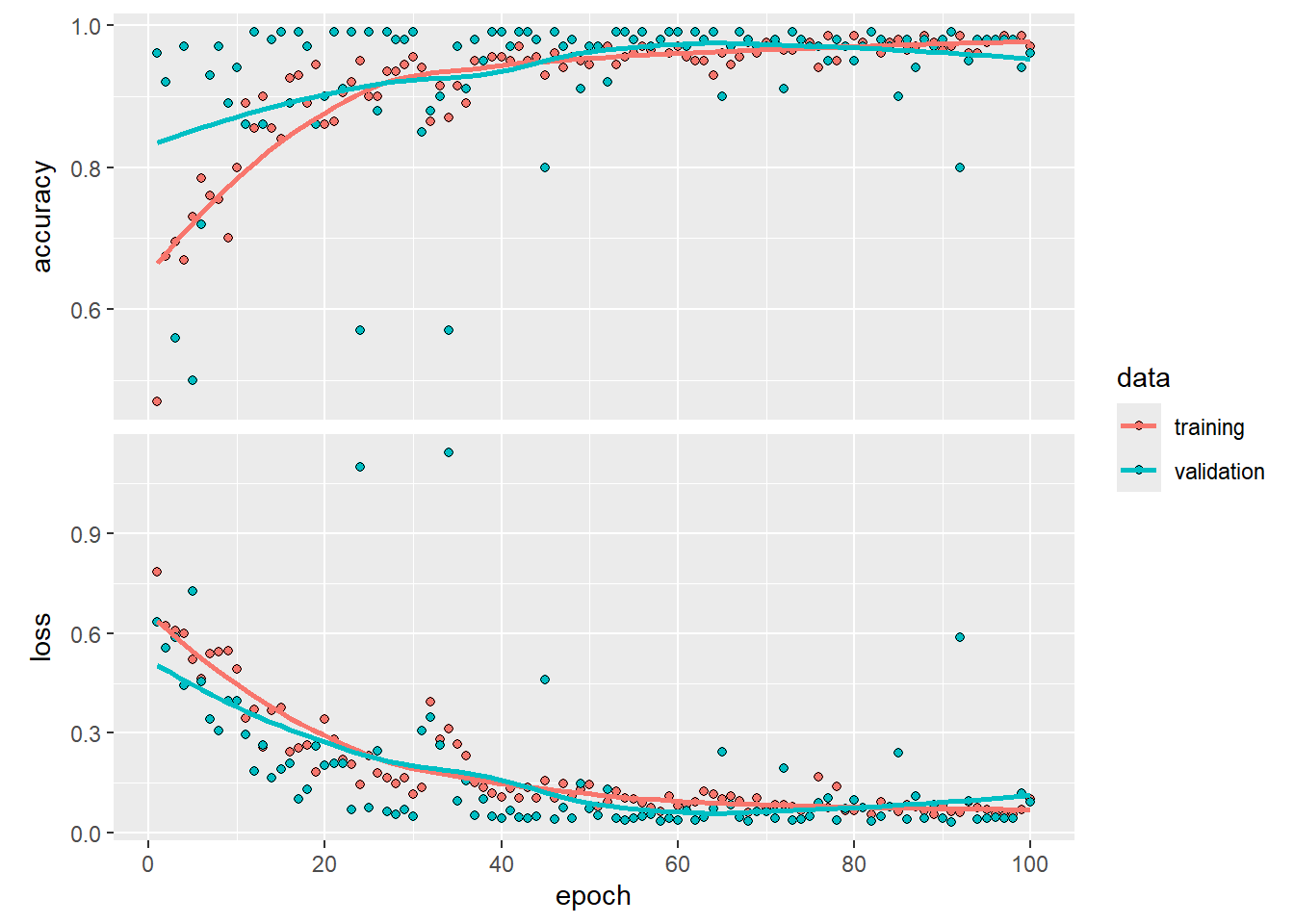
plot(history)
Well, that doesn’t look too bad for a first try with only a small
model. Eventually the accuracy on our validation set reaches more than
90%, but this took quite a number of epochs and the performance doesn’t
look very stable. Given that everyone has different training and
validation data, your results may of course be different. It is very
likely that with this current model architecture your model will even
not be able to make good predictions at all on the validation (or even
train) set. Don’t worry if that’s the case for you. But hang on, is it
really a small model?
Our small model still has almost 20 thousand parameters that were
trained… This is of course way more than what is common for general
frequentist models, but for a CNN it is indeed still small.
However, we see that especially in our last dense layer many parameters
were involved. If we were to reduce the size of the feature vector that
is used as the input of the final layer, then we can substantially
reduce our number of parameters. So let’s see if we can set up a CNN
with a bit smarter architecture that has too train fewer parameters and
focuses more on the most important patterns. Hopefully this will
stabilize and increase our performance.
As you may remember from the second practical, we can reduce the size
of our data with a pooling layer. Let’s try this now.
Exercise 16.4b
Create a new model (called model2), but now after the
convolution layer add a max pooling layer with a kernel size of 3 by 3.
Moreover, because we are now pooling before flattening the feature
vector, you can increase the number of filters in the first
convolutional layer to 20 and probably still have fewer trainable
parameters than the first model had.
Make sure to compile and fit the model again. Save the output as
history2 and visualize this afterwards.
How many trainable parameters will this new CNN have?
Great, that looks better! Especially considering that this model is
smaller in terms of trainable parameters, but that at the same time it
also results in a higher performance on the validation set. Moreover,
the improvement in the loss/cost-function increases faster and more
stable over the epochs than during the fitting of the first model. This
indicates that this model is actually focusing its learning on more
important parameters. Let’s see if we can improve it a bit more,
especially if the variation in the validation accuracy over the epochs
can be improved even further. Adding one or two extra convolution layer
will not add a lot of extra parameters to our model, especially not if
we also add one or two dropout layers to it as well. However, with these
extra convolution layers the model will be able to detect more
complicated (higher-order) patterns in the images than (for example)
edges.
Try to add one or two convolution layers to the model and run it
again. You can add these before or after the max pooling layer, note how
this will impact your number of parameters. Add a drop-out layer after
the last (or perhaps even each) convolution layer with a drop rate of
for example 0.2 to reduce the number of parameters. You can also change
the number of filters for the different convolution layers to see if
that improves the performance. Finally, because we convolve multiple
times, the images will lose quite some number of pixels from their edges
in the final layers (remember from the previous practical?). To prevent
this add padding = "same" as an argument to the convolution
layers. This will create an extra layer of zeroes around the images
before executing the convolution, which will result in the same
dimension of output images as the input.
See if the performance has improved in this 3rd model:
do the accuracies show a small spread?
do the accuracies quickly improve over the epochs?
are the training and validation accuracies in the same range?
do the accuracies reach an asymptote?
are the accuracies close to 100%?
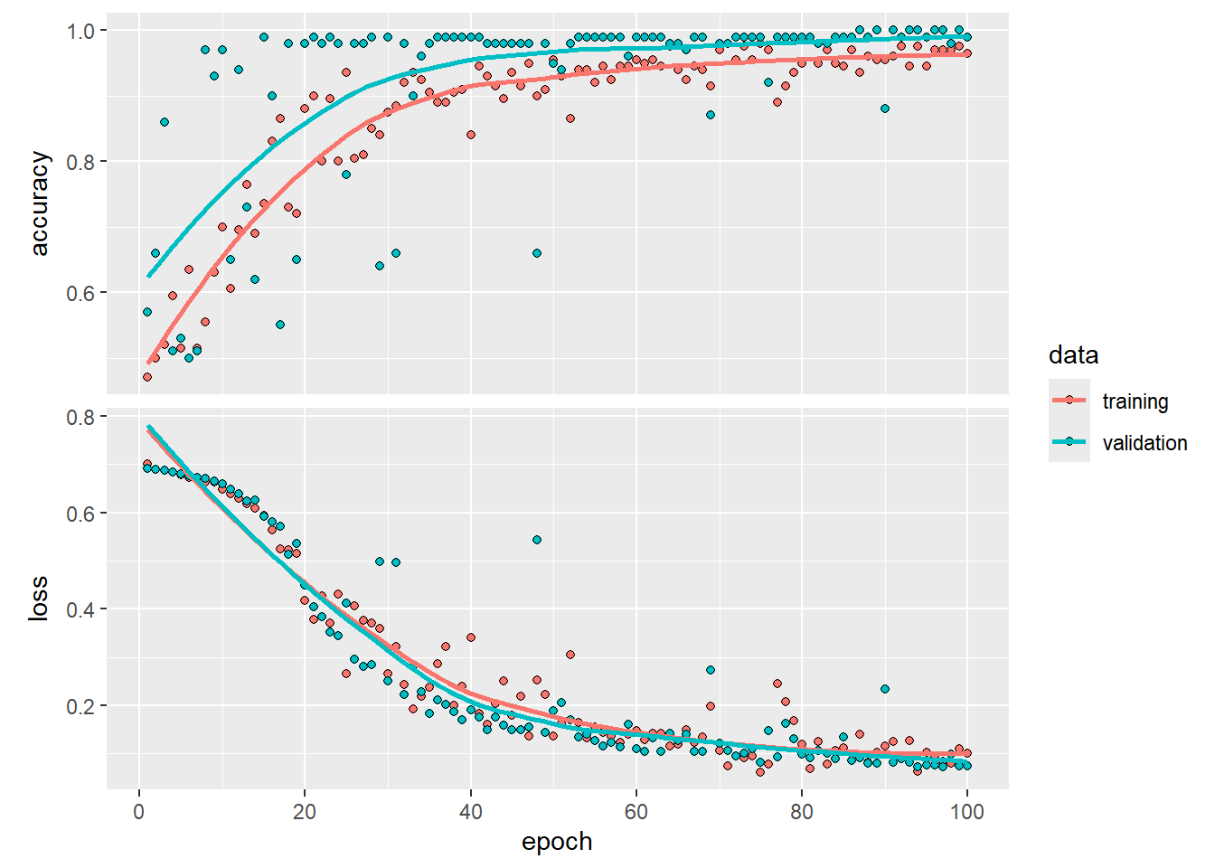
The below model is our own try, how does this look compared to your
own?
As you can see, although our third model has a lot more layers, it
has by far the fewest trainable parameters. Moreover, it showed a steady
increase in performance over the epochs, but unfortunately with still a
few outliers to lower performance here and there. Furthermore, it is
clearly learning slower than the second model did and it seems that it
did not level off completely yet. Probably with some extra epochs it
could have improved even further.
Although the third model can still be improved, we’re happy enough
with the stable increase in performance over the epochs for both the
train and validation set and especially with the performance on the
validation set for the final few epochs. Therefore we apply this last
model on our test image.
Exercise 16.5a
Why do we want to apply the model on a test image?
It could be that the model is overfitted on our validation image, for
example because our annotated examples did not include enough
variation.
We have not labelled any of our test grid cells, but visualizing
which grid cells our model predicts to be bush and which not will be
very useful to visually check for the generalizability of the model.
Let’s do that now. To do that we can add one line of code to generate
the predictions on the test set.
# Predict fitted CNN on test data
testpred <- model3 %>%
  predict(testx)
## 158/158 - 1s - 4ms/step
Exercise 16.5b
Now we’re going to visualize the grid cells of the two predicted
classes in the test image. You have been working and thinking very hard
until this point, so we’re going to make life a little bit easier for
you by supplying the code to plot the test image classes for you. Try to
copy and paste this code to run it for yourself.
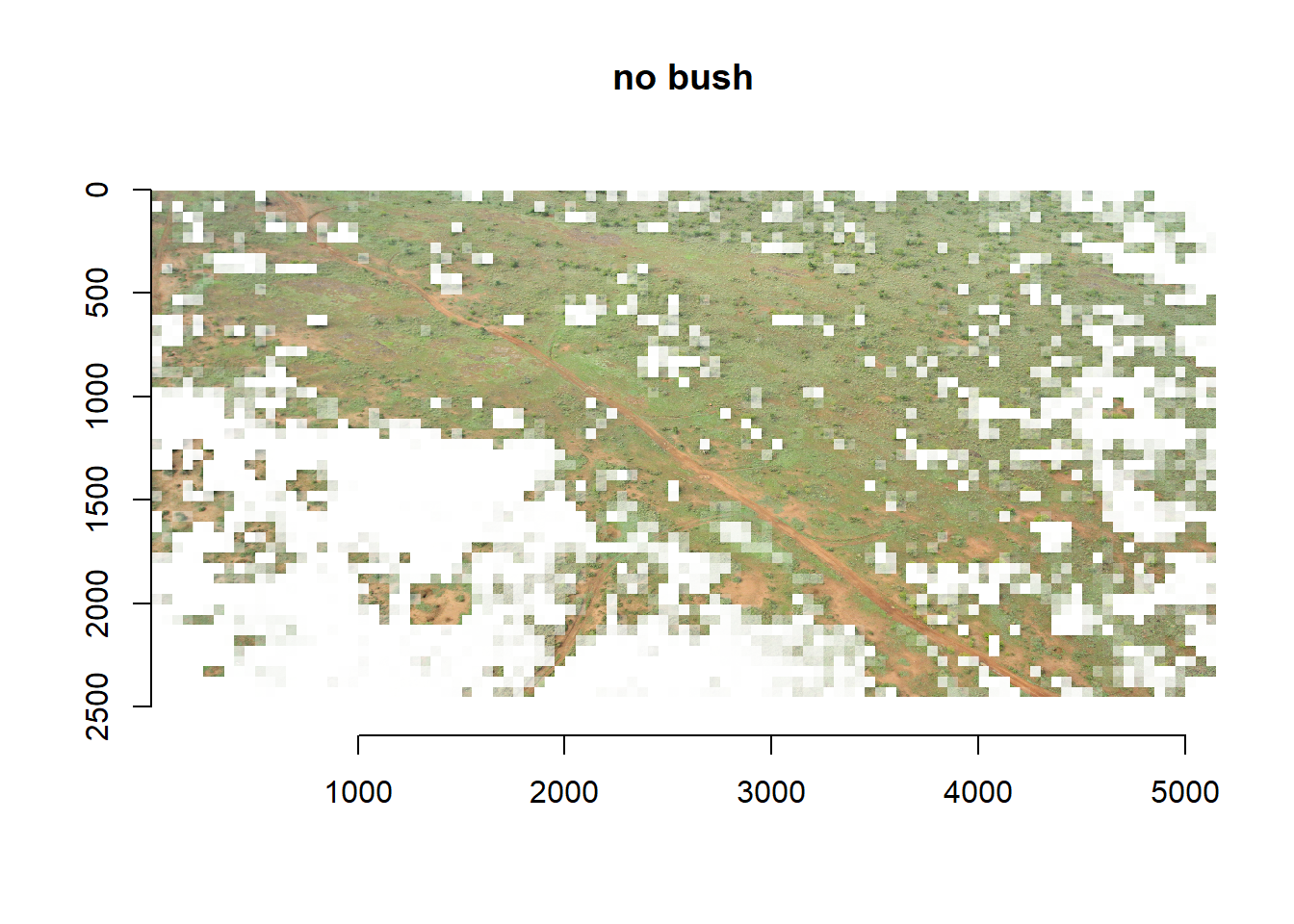
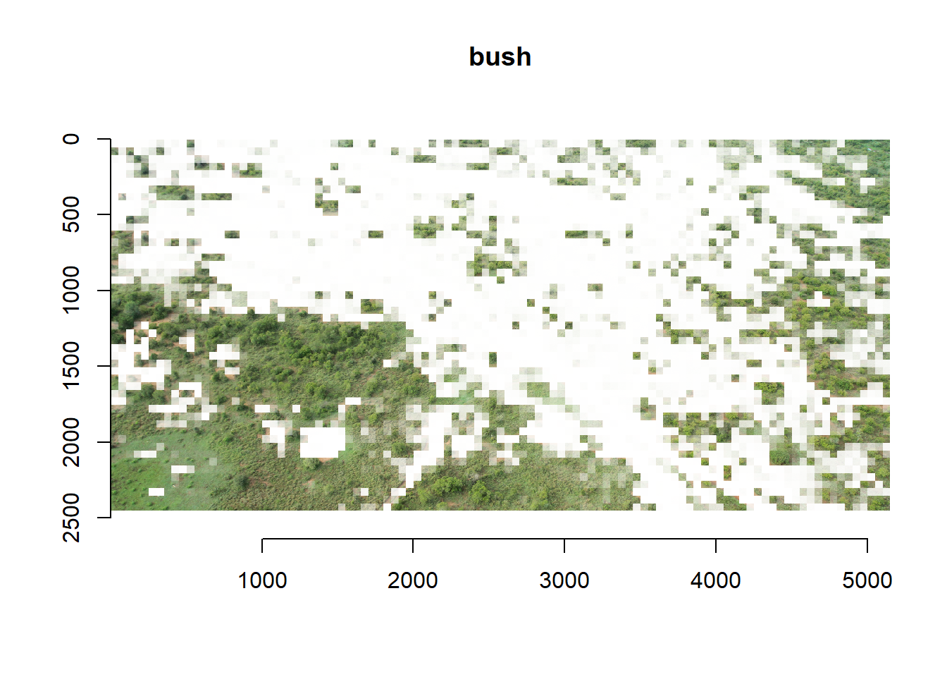
With the following code you will make two copies of the test grid
cells (one image for bush and one for the other class) and make the
cell’s transparency inversely proportional to the probability of the
predicted class. After that you determine (using your original test
image) how many grid cells fitted in both the x- and y- dimension, you
can check if these numbers are correct by inspecting the filenames of
the grid cells in your test-folder. Then you split the
imlist into equal chunks, where each sublist contains all
the grid cells of one row in the image. Please note that the order in
which you should do this depends on the order in which you supplied your
grid cells to the testx object in the first place. If you
did this per column instead of per row, then you should of course also
evaluate the predictions per column. Finally, you paste all the grid
cells together again per row (in the loop) and then all the rows
together after that.
Not bad… We can see that what is bush is generally predicted as bush
and what is not bush is also predicted as such. However, we do see that
especially in the lower left corner a lot of presumably high shrubs or
grass are predicted as bush. Furthermore, some small bushes that are not
connected to other bushes are wrongly classified as not being bush. This
last issue could probably be an artefact of the regular grid cells that
might be too large for these bushes or that cut them in half. Still, not
a result to be ashamed of!
6 Conclusion
Well, actually there is not really a conclusion here. Some stories
have an open ending, just like this practical. We have created quite a
good model already, with a good accuracy on the validation set and
sensible results on the test set. However, we’ve also seen that the test
set contains some predictions that could have been better.
7 Challenge
Challenge
Now see if you can beat our model… Check if you can for example
correctly identify the grid cells on the bottom left corner of the test
image. Or see if you can create a more stable accuracy and loss output
for the validation set. Or see if you can achieve the same performance
with a simpler model. Or go nuts and create a very complicated model.
There are a lot more switches and levers that you can tweak in the CNN.
We haven’t for example optimized our batch size and learning rate. Also
think about the final layer, after the flattening we immediately
predicted the two classes, see if some extra hidden dense layers will
improve the performance. Maybe try different optimizer algorithms, a
different loss function, or add learning rate decay functions. Take a
look at the keras tutorials again and look at the help files of
the functions to see what you can tweak. Finally, and maybe most
importantly: take a look at your training and validation data! Do you
have enough training records and do this data have enough variation per
class? Updating the labels can maybe improve the performance of the
model as well, especially on the patch in the bottom left of the test
image.
To do all this, try to create a script where you loop over multiple
combinations of hyperparameter values to optimize the performance of
your CNN (so using a grid search). You can do this by for example
creating a data.frame or tibble with all
combinations of hyperparameter values (by using the handy
expand.grid). Then create a for loop that loops over all
the rows in this data.frame or tibble that uses the set values for the
hyperparameters at the corresponding iteration of the loop. Just don’t
forget to save the output during each iteration of the loop, or
otherwise it will be a shame of your time and CPU sweat and tears (not
talking out of experience here of course…).
Please let us know what you come up with, we’re always happy to learn
from you… And above all: enjoy!
8 Submit your last plot
Submit your script file as well as a plot: either your last created
plot, or a plot that best captures your solution to the challenge.
Submit the files on Brightspace via Assessment > Assignments >
Skills day 16.
Note that your submission will not be graded or
evaluated. It is used only to facilitate interaction and to get insight
into progress.
9 Recap
Today, we’ve finally fitted a CNN to the image data that we prepared
the last days. By first cutting the original images into many
(thousands) of smaller 50x50 pixel tiles, and then training a CNN
image classifier to the sets of bush vs other
classes, we’ve in some sense implemented segmentation of the full image
by classifying all smaller tiles into the two classes.
An R script of today’s exercises can be downloaded
here