To specify a formula, use the function recipe; to remove
columns use step_rm; to center use
step_center; to scale use step_scale. To
prepare the data recipe use the prep function (this will
then automatically use the data passed on to the recipe
function for training the data recipe (thus, here the
training data!). Put all steps behind each other in one
sequences using pipes.
Supervised learning
Overview
Today’s goal: to apply supervised learning algorithms to the cattle time series data.
Resources
- Tutorial 9
- Tidy Modeling with R
- A gentle introduction to tidymodels
- Modelling with tidymodels and parsnip
- Algorithms supported by parship
Packages
tidymodels, consisting of: rsample, recipes, parsnip and yardstick, but also: kernlab and randomForest
Main functions
group_vfold_cv, analysis,
assessment, recipe, prep,
bake, svm_rbf, rand_forest,
set_engine, fit, predict,
metrics, pr_curve, workflow
1 Introduction
Yesterday we applied some unsupervised machine learning algorithms,
today we will be applying two types of supervised machine learning
algorithms: Support Vector Machines (SVM) and Random Forests (RF). We
will continue with the cattle movement data that we worked with the last
2 days. Because we had the column label in the dataset,
which contained the annotated behaviour based on direct visual
observation, we have a labelled dataset and thus possibility to use
supervised learning.
Recall from the lecture on the data science workflow that in predictive modelling it is necessary to split the data into train and validation set. This can be done randomly, but this should only be done with great care. As we are dealing with time series data on individual animals, which generally have high degrees of temporal autocorrelation, randomly splitting the data into train and validation sets is not making sure that both sets are independent! In tutorial 9 we called non-independent train and validation sets a form of data leakage, in which by mistake information is shared between the training and validation data sets. In general, by dividing a set of data into training and validation sets, the goal is to ensure that no data is shared between the two.
Thus, it may be better to keep all the data of a specific individual together, and allocate all data from a single individual (or time-series) to either the train dataset or the validation dataset. Such partitioning of the data into train and validation sets can be done once, or using a k-fold cross validation approach. We will use both here.
Exercise 13.1a
Download the file dat_ts2.rds from Brightspace >
Time series analyses > datasets > cattle, and store in an
appropriate folder (e.g. data / processed / cattle /). Load the
file into an object called dat. Note that it is an .rds
file, which can be read into R with the function read_rds
(see tutorial 1). Also load (and install if needed) the packages
tidyverse, tidymodels and kernlab. library(tidyverse)
library(tidymodels)
library(kernlab)
dat <- readRDS("data/processed/cattle/dat_ts2.rds")
dat## # A tibble: 2,159 × 12
## IDburst isGrazing xacc_mean xacc_sd yacc_mean yacc_sd zacc_mean zacc_sd VeDBA_mean VeDBA_sd step angle
## <fct> <fct> <dbl> <dbl> <dbl> <dbl> <dbl> <dbl> <dbl> <dbl> <dbl> <dbl>
## 1 1_1 TRUE -6.06 13.5 -34.7 21.9 -13.0 19.8 46.2 17.8 0.199 0.983
## 2 1_1 TRUE -1.91 18.8 -30.4 27.7 -7.80 22.5 46.9 20.2 0.109 -0.250
## 3 1_1 TRUE -7.59 14.7 -23.5 25.3 -3.15 21.5 40.5 16.9 0.0892 0.619
## 4 1_1 TRUE -8.88 13.3 -18.8 12.6 -4.31 11.8 28.5 10.5 0.204 -0.894
## 5 1_1 TRUE -1.75 22.4 -19.6 23.6 -5.09 21.1 40.3 16.7 0.0486 -0.444
## 6 1_1 TRUE -4.60 16.8 -23.2 22.8 -1.83 15.0 35.8 17.5 0.167 0.236
## 7 1_1 TRUE -6.55 15.1 -15.2 21.4 -2.14 16.2 30.8 16.6 0.453 0.958
## 8 1_1 TRUE -6.04 16.6 -27.0 28.1 -9.91 24.3 45.6 20.6 0.379 0.977
## 9 1_1 TRUE -7.10 13.4 -23.5 28.3 -6.14 21.4 41.1 19.3 0.243 0.996
## 10 1_1 TRUE -11.4 9.62 -19.8 17.4 -5.07 13.8 31.3 12.1 0.220 0.976
## # ℹ 2,149 more rowsThe data dat does not have the column label
like we had in the previous 2 tutorials; here it is reclassified to the
new column isGrazing, which is a factor with 2
levels indicating whether or not the cows were grazing.
For your information, the dataset loaded above was created from the dataset “dat_ts1.rds” loaded yesterday via the following chain of dplyr functions:
read_rds("data/processed/cattle/dat_ts1.rds") %>%
  select(-c(dttm,t,x,y,dx,dy,head)) %>%
  unite(IDburst, c(ID, burst)) %>%
  drop_na(angle) %>%
  mutate(angle = cos(angle),
         IDburst = as.factor(IDburst),
         isGrazing = as.factor(label == "grazing")) %>%
  select(-label) %>%
  select(IDburst, isGrazing, everything()) # just for reordering columns
2 Splitting the data
The rsample package, part of tidymodels,
offers functions to split the data into different sets (e.g. for
training and testing). In tutorial 9 we already saw the simple
initial_split function that partitions the data randomly
into 2 parts. However, because this function randomly allocates records
to either of the datasets, and not a grouped set of records
(e.g. belonging to the same individual, or timeseries thereof), we can
better not use this function here.
Exercise 13.2a
Check the helpfile of the group_initial_split function and
create a train-test split based on grouping variable
IDburst, where you specify that ca 75% of the data should
be assigned to the training dataset, and the rest to the test dataset.
Assign the result to an object called main_split and check
the object by printing it to the console main_split <- group_initial_split(dat, group = IDburst, prop = 3/4)
main_split## <Training/Testing/Total>
## <1551/608/2159>We now have splitted the data in 2 parts: 1 part can be used for
model development (here ca 75%) , whereas the other part (here ca 25%)
can be used for testing the model predictions. In a data science project
involving machine learning, model development is often done
using k-fold cross validation, where both trainable parameters
are learned but also hyperparameters are tuned. To do k-fold
cross validation with groups, we can use the group_vfold_cv
function, which is a function that creates splits of the data based on
some grouping variable in a k-fold (here called
V-fold) cross-validation approach.
Exercise 13.2b
Check the helpfile of the group_vfold_cv function. Retrieve
the training data from the object main_split
created above (remember from earlier that the function
training can be used here), and with the training data
create a train-validation split with 5 folds based on grouping variable
IDburst. Assign the result to an object called
dat_split and check the object by printing it to the
screen. dat_split <- group_vfold_cv(training(main_split), group = IDburst, v = 5)
dat_split## # Group 5-fold cross-validation
## # A tibble: 5 × 2
## splits id
## <list> <chr>
## 1 <split [1165/386]> Resample1
## 2 <split [1212/339]> Resample2
## 3 <split [1237/314]> Resample3
## 4 <split [1227/324]> Resample4
## 5 <split [1363/188]> Resample5You’ll see that the output of group_vfold_cv is a
tibble, here with 5 rows (as we set it to 5 folds), in which the first
column, splits, is a named list with split data. it shows
the number of records in the train dataset, and in the validation
dataset, for each fold. Using the function analysis, we can
extract the data to be used for training, whereas with the
assessment function we can extract the data that should be
used for validation. To retrieve the first record/fold of the data
splits, we can use dat_split$splits[[1]].
Exercise 13.2c
Extract the train and validation data for the first fold, and assign
these to the objects dat_train and dat_val,
respectively. Print the objects to the console so you can inspect them.
dat_train <- analysis(dat_split$splits[[1]])
dat_val   <- assessment(dat_split$splits[[1]])
dat_train
## # A tibble: 1,165 × 12
## IDburst isGrazing xacc_mean xacc_sd yacc_mean yacc_sd zacc_mean zacc_sd VeDBA_mean VeDBA_sd step angle
## <fct> <fct> <dbl> <dbl> <dbl> <dbl> <dbl> <dbl> <dbl> <dbl> <dbl> <dbl>
## 1 1_1 TRUE -6.06 13.5 -34.7 21.9 -13.0 19.8 46.2 17.8 0.199 0.983
## 2 1_1 TRUE -1.91 18.8 -30.4 27.7 -7.80 22.5 46.9 20.2 0.109 -0.250
## 3 1_1 TRUE -7.59 14.7 -23.5 25.3 -3.15 21.5 40.5 16.9 0.0892 0.619
## 4 1_1 TRUE -8.88 13.3 -18.8 12.6 -4.31 11.8 28.5 10.5 0.204 -0.894
## 5 1_1 TRUE -1.75 22.4 -19.6 23.6 -5.09 21.1 40.3 16.7 0.0486 -0.444
## 6 1_1 TRUE -4.60 16.8 -23.2 22.8 -1.83 15.0 35.8 17.5 0.167 0.236
## 7 1_1 TRUE -6.55 15.1 -15.2 21.4 -2.14 16.2 30.8 16.6 0.453 0.958
## 8 1_1 TRUE -6.04 16.6 -27.0 28.1 -9.91 24.3 45.6 20.6 0.379 0.977
## 9 1_1 TRUE -7.10 13.4 -23.5 28.3 -6.14 21.4 41.1 19.3 0.243 0.996
## 10 1_1 TRUE -11.4 9.62 -19.8 17.4 -5.07 13.8 31.3 12.1 0.220 0.976
## # ℹ 1,155 more rowsdat_val## # A tibble: 386 × 12
## IDburst isGrazing xacc_mean xacc_sd yacc_mean yacc_sd zacc_mean zacc_sd VeDBA_mean VeDBA_sd step angle
## <fct> <fct> <dbl> <dbl> <dbl> <dbl> <dbl> <dbl> <dbl> <dbl> <dbl> <dbl>
## 1 8_1 TRUE 10.1 12.0 -16.1 26.7 -0.0563 22.4 37.6 17.2 0.142 0.930
## 2 8_1 TRUE 4.53 18.9 -19.3 21.8 1.31 23.9 38.7 17.0 0.191 0.996
## 3 8_1 TRUE 2.34 18.9 -14.6 21.2 1.18 27.6 40.1 12.7 0.300 0.995
## 4 8_1 TRUE 6.46 11.8 -10.1 16.0 6.12 14.9 26.3 10.2 0.467 -1.000
## 5 8_1 TRUE 4.22 13.9 -12.7 12.9 6.40 9.68 23.8 10.3 0.241 -0.411
## 6 8_1 TRUE 0.129 13.1 -22.0 16.4 -3.21 14.5 31.8 11.3 0.247 0.923
## 7 8_1 TRUE 1.60 11.0 -15.5 14.4 -0.629 11.5 24.4 10.5 0.655 -0.887
## 8 8_1 TRUE 0.0357 19.4 -17.4 24.9 2.54 24.5 38.3 20.6 0.298 0.493
## 9 8_1 TRUE 4.90 13.3 -15.9 13.3 1.13 14.7 27.0 10.7 0.431 0.860
## 10 8_1 TRUE 7.11 10.1 -11.8 9.70 2.62 7.35 19.2 8.79 0.520 0.996
## # ℹ 376 more rows3 Create data recipe
Using the rsample package we have splitted the data into
k folds used for training and validation, now we will proceed
and use the recipes package to set up a data recipe.
Recall from tutorial 9 that a data recipe is a description of what steps
should be applied to a data set in order to get it ready for data
analysis. Most steps in the recipe are defined using functions that
start with the prefix step_.
Exercise 13.3a
Create a data recipe called dataRecipe that:
- takes the training data as input;
- specifies that the formula for the analyses is
isGrazing ~ .; - removes the column
IDburstfrom the data; - centers all predictors;
- scales all predictors;
- prepares the data recipe using the training data.
dataRecipe <- dat_train %>%
  recipe(isGrazing ~ .) %>%
  step_rm(IDburst) %>%
  step_center(all_predictors()) %>%
  step_scale(all_predictors()) %>%
  prep()
dataRecipe
4 Bake data
Now that we have splitted the data into train and validation set, and now that we’ve set up and prepared a data recipe, let’s bake some data: recipes metaphor for apply the preprocessing computations to new data.
Exercise 13.4a
Bake the dataset dat_train and do the same for the
dat_val dataset. Assign the results to objects called
baked_train and baked_val, respectively.
baked_train  <- dataRecipe %>%
  bake(dat_train)
baked_train
## # A tibble: 1,165 × 11
## xacc_mean xacc_sd yacc_mean yacc_sd zacc_mean zacc_sd VeDBA_mean VeDBA_sd step angle isGrazing
## <dbl> <dbl> <dbl> <dbl> <dbl> <dbl> <dbl> <dbl> <dbl> <dbl> <fct>
## 1 -1.06 -0.0994 -1.64 0.701 -2.75 0.385 1.14 1.13 -0.422 0.918 TRUE
## 2 -0.295 0.883 -1.45 1.52 -1.67 0.741 1.20 1.65 -0.563 -0.967 TRUE
## 3 -1.34 0.127 -1.13 1.18 -0.698 0.607 0.627 0.945 -0.595 0.362 TRUE
## 4 -1.58 -0.131 -0.914 -0.596 -0.939 -0.672 -0.444 -0.431 -0.414 -1.95 TRUE
## 5 -0.265 1.56 -0.951 0.945 -1.10 0.557 0.613 0.903 -0.659 -1.26 TRUE
## 6 -0.792 0.519 -1.12 0.835 -0.421 -0.253 0.203 1.07 -0.473 -0.224 TRUE
## 7 -1.15 0.205 -0.749 0.635 -0.487 -0.0890 -0.242 0.867 -0.0232 0.881 TRUE
## 8 -1.06 0.479 -1.29 1.57 -2.11 0.980 1.09 1.73 -0.139 0.909 TRUE
## 9 -1.25 -0.114 -1.13 1.60 -1.32 0.592 0.684 1.46 -0.354 0.939 TRUE
## 10 -2.05 -0.822 -0.959 0.0667 -1.10 -0.406 -0.195 -0.0760 -0.390 0.908 TRUE
## # ℹ 1,155 more rowsbaked_val <- dataRecipe %>%
bake(dat_val)
baked_val## # A tibble: 386 × 11
## xacc_mean xacc_sd yacc_mean yacc_sd zacc_mean zacc_sd VeDBA_mean VeDBA_sd step angle isGrazing
## <dbl> <dbl> <dbl> <dbl> <dbl> <dbl> <dbl> <dbl> <dbl> <dbl> <fct>
## 1 1.93 -0.380 -0.788 1.38 -0.0512 0.723 0.365 0.999 -0.512 0.838 TRUE
## 2 0.894 0.906 -0.938 0.683 0.234 0.926 0.467 0.952 -0.434 0.939 TRUE
## 3 0.490 0.905 -0.722 0.598 0.208 1.41 0.594 0.0475 -0.264 0.937 TRUE
## 4 1.25 -0.423 -0.514 -0.120 1.24 -0.264 -0.649 -0.486 -0.000425 -2.11 TRUE
## 5 0.838 -0.0215 -0.634 -0.554 1.30 -0.958 -0.873 -0.464 -0.356 -1.21 TRUE
## 6 0.0819 -0.171 -1.06 -0.0690 -0.711 -0.323 -0.153 -0.263 -0.347 0.827 TRUE
## 7 0.353 -0.556 -0.762 -0.343 -0.171 -0.711 -0.818 -0.436 0.295 -1.94 TRUE
## 8 0.0646 0.994 -0.850 1.12 0.491 0.999 0.428 1.72 -0.267 0.169 TRUE
## 9 0.963 -0.140 -0.781 -0.507 0.197 -0.291 -0.585 -0.380 -0.0565 0.731 TRUE
## 10 1.37 -0.725 -0.591 -1.01 0.508 -1.27 -1.28 -0.792 0.0823 0.938 TRUE
## # ℹ 376 more rows5 Define and train the model
Now that all data is properly pre-processed we can proceed to train a model/algorithm. Recall from tutorial 9 that a model is trained using the parsnip package, by first defining the model, then specifying the engine that will execute the model estimation for us, and finally fitting the model. Which models currently are supported and via which function they should be defined can be seen here. We will focus on a Support Vector Machine, SVM, and specifically a SVM with a Gaussian radial basis function.
A SVM with a Gaussian radial basis function can be specified in the
parsnip package via the svm_rbf function. For a
classification problem (i.e. our machine learning task of classifying
the annotated behaviour), it takes 3 arguments: mode which
should be set to "classification", as well as the
hyperparameters cost and rbf_sigma. Check the
helpfile for information on these parameters.
Exercise 13.5a
Fit a SVM to the train data baked_train. Do this by
first specifying the model: specify it to be a classification mode, with
cost parameters set to value 1.0, and
rbf_sigma parameter set to value 0.001 Then, set the engine
to "kernlab". Finally, fit the model using the formula
isGrazing ~ . (i.e. isGrazing is the response,
and all other columns are predictors) with data
baked_train. Assign the fitted model to an object called
dat_SVMfit.
Specify the model using svm_rbf, then set the engine
using set_engine, and fit the model using
fit.
dat_SVMfit <- svm_rbf(mode = "classification",
                      cost = 1.0,
                      rbf_sigma = 0.001) %>%
  set_engine("kernlab") %>%
  fit(isGrazing ~ ., data = baked_train)
dat_SVMfit
## parsnip model object
##
## Support Vector Machine object of class "ksvm"
##
## SV type: C-svc (classification)
## parameter : cost C = 1
##
## Gaussian Radial Basis kernel function.
## Hyperparameter : sigma = 0.001
##
## Number of Support Vectors : 319
##
## Objective Function Value : -265.9519
## Training error : 0.084979
## Probability model included.6 Making predictions
With the fitted model stored in object dat_SVMfit, we
can now predict the model on the validation dataset
baked_val using the predict function. The
function by default returns the predicted class, but we can also
retrieve the predicted classes and probabilities by adding the function
argument type = "prob" (then fitted using parsnip; the
column names will then be .pred_FALSE and
.pred_TRUE), or type = "probabilities" (when
fitted directly using kernlab; the column names will then be
FALSE and TRUE).
Exercise 13.6a
Predict the fitted SVM on the baked_val validation dataset:
predict the class probabilities, and save to an object
dat_preds. Also add the columns of dat_val
using the function bind_cols. Because we predict
probabilities, and because our response variable isGrazing
is a factor with levels "TRUE" and
"FALSE", we get as predictions the columns
".pred_FALSE" and ".pred_TRUE". dat_preds <- dat_SVMfit %>%
predict(baked_val, type = "prob") %>%
bind_cols(dat_val)
dat_preds## # A tibble: 386 × 14
## .pred_FALSE .pred_TRUE IDburst isGrazing xacc_mean xacc_sd yacc_mean yacc_sd zacc_mean zacc_sd VeDBA_mean VeDBA_sd step angle
## <dbl> <dbl> <fct> <fct> <dbl> <dbl> <dbl> <dbl> <dbl> <dbl> <dbl> <dbl> <dbl> <dbl>
## 1 0.0182 0.982 8_1 TRUE 10.1 12.0 -16.1 26.7 -0.0563 22.4 37.6 17.2 0.142 0.930
## 2 0.0181 0.982 8_1 TRUE 4.53 18.9 -19.3 21.8 1.31 23.9 38.7 17.0 0.191 0.996
## 3 0.0283 0.972 8_1 TRUE 2.34 18.9 -14.6 21.2 1.18 27.6 40.1 12.7 0.300 0.995
## 4 0.0833 0.917 8_1 TRUE 6.46 11.8 -10.1 16.0 6.12 14.9 26.3 10.2 0.467 -1.000
## 5 0.0786 0.921 8_1 TRUE 4.22 13.9 -12.7 12.9 6.40 9.68 23.8 10.3 0.241 -0.411
## 6 0.0430 0.957 8_1 TRUE 0.129 13.1 -22.0 16.4 -3.21 14.5 31.8 11.3 0.247 0.923
## 7 0.0762 0.924 8_1 TRUE 1.60 11.0 -15.5 14.4 -0.629 11.5 24.4 10.5 0.655 -0.887
## 8 0.0171 0.983 8_1 TRUE 0.0357 19.4 -17.4 24.9 2.54 24.5 38.3 20.6 0.298 0.493
## 9 0.0613 0.939 8_1 TRUE 4.90 13.3 -15.9 13.3 1.13 14.7 27.0 10.7 0.431 0.860
## 10 0.121 0.879 8_1 TRUE 7.11 10.1 -11.8 9.70 2.62 7.35 19.2 8.79 0.520 0.996
## # ℹ 376 more rows
Exercise 13.6b
Let’s also add not just the predicted probabilities of both classes, but the predicted class itself. You can do so by adding the prediction column using :
dat_preds <- dat_preds %>%
bind_cols(predict(dat_SVMfit, baked_val, type = "class"))isGrazing,
which is a factor with levels "TRUE" and
"FALSE", the newly created column “.pred_class” also is a
factor with these levels! dat_preds <- dat_preds %>%
bind_cols(predict(dat_SVMfit, baked_val, type = "class"))
dat_preds## # A tibble: 386 × 15
## .pred_FALSE .pred_TRUE IDburst isGrazing xacc_mean xacc_sd yacc_mean yacc_sd zacc_mean zacc_sd VeDBA_mean VeDBA_sd step angle .pred_class
## <dbl> <dbl> <fct> <fct> <dbl> <dbl> <dbl> <dbl> <dbl> <dbl> <dbl> <dbl> <dbl> <dbl> <fct>
## 1 0.0182 0.982 8_1 TRUE 10.1 12.0 -16.1 26.7 -0.0563 22.4 37.6 17.2 0.142 0.930 TRUE
## 2 0.0181 0.982 8_1 TRUE 4.53 18.9 -19.3 21.8 1.31 23.9 38.7 17.0 0.191 0.996 TRUE
## 3 0.0283 0.972 8_1 TRUE 2.34 18.9 -14.6 21.2 1.18 27.6 40.1 12.7 0.300 0.995 TRUE
## 4 0.0833 0.917 8_1 TRUE 6.46 11.8 -10.1 16.0 6.12 14.9 26.3 10.2 0.467 -1.000 TRUE
## 5 0.0786 0.921 8_1 TRUE 4.22 13.9 -12.7 12.9 6.40 9.68 23.8 10.3 0.241 -0.411 TRUE
## 6 0.0430 0.957 8_1 TRUE 0.129 13.1 -22.0 16.4 -3.21 14.5 31.8 11.3 0.247 0.923 TRUE
## 7 0.0762 0.924 8_1 TRUE 1.60 11.0 -15.5 14.4 -0.629 11.5 24.4 10.5 0.655 -0.887 TRUE
## 8 0.0171 0.983 8_1 TRUE 0.0357 19.4 -17.4 24.9 2.54 24.5 38.3 20.6 0.298 0.493 TRUE
## 9 0.0613 0.939 8_1 TRUE 4.90 13.3 -15.9 13.3 1.13 14.7 27.0 10.7 0.431 0.860 TRUE
## 10 0.121 0.879 8_1 TRUE 7.11 10.1 -11.8 9.70 2.62 7.35 19.2 8.79 0.520 0.996 TRUE
## # ℹ 376 more rows7 Evaluating model predictions
After model fitting and prediction using parsnip, we can use
the functions from the package yardstick to compute
model evaluation metrics. The metrics function can be used
for this, taking input arguments truth and
estimate (which should be the predicted class, and not the
predicted class probability!). For example, the following code will
compute model evaluation metrics based on a classification problem:
Exercise 13.7a
Compute the metrics for the fitted model, using column “isGrazing” as
the true label, and the column with the predicted class as the estimate.
dat_preds %>%
  metrics(truth = isGrazing,
          estimate = .pred_class)
## # A tibble: 2 × 3
## .metric .estimator .estimate
## <chr> <chr> <dbl>
## 1 accuracy binary 0.751
## 2 kap binary 0.474The results are estimates for the accuracy and
kappa statistic for the model prediction. The accuracy is quite
high: around 75% of the labels have been correctly predicted! To see how
the predictions are for both classes, we can compute the confusion
matrix the conf_mat function:
dat_preds %>%
  conf_mat(truth = isGrazing,
           estimate = .pred_class)
## Truth
## Prediction FALSE TRUE
## FALSE 83 5
## TRUE 91 207We see that most of the records where the cattle did or
did not graze were correctly classified as such. In this case,
207 of the 212 records were the cattle were in fact grazing were
correctly classified as such (recall: ca 98%), whereas 207 of
the 298 records were cattle were predicted to be grazing they were in
indeed also doing that (precision: ca 71%). As mentiond in the
lectures, instead of simply being interested in accuracy only,
we are often interested in these precision and recall
metrics of model predictions. See
here
for a good overview of what these (and other) measures mean (reading
material for the lecture on the data science workflow). the yardstick
package offers the function pr_curve to compute the
precision and recall along a gradient in threshold values.
Exercise 13.7b
Compute the precision and recall using the function
pr_curve. Do this based on the data dat_preds
(in 13.6 you have added the class predictions), using
isGrazing as the true label, and .pred_TRUE
(or TRUE if you did not use parsnip for model fitting but
rather kernlab directly) as the predicted value, and set the
“event_level” argument to value “second” (namely, from FALSE and TRUE,
the second value is the focus). Assign the result to an object
called PR, inspect it by printing it to the screen, and
plot PR using the autoplot function. PR <- dat_preds %>%
pr_curve(truth = isGrazing, .pred_TRUE, event_level = "second")
PR## # A tibble: 387 × 3
## .threshold recall precision
## <dbl> <dbl> <dbl>
## 1 Inf 0 1
## 2 0.990 0.00472 1
## 3 0.990 0.00943 1
## 4 0.990 0.0142 1
## 5 0.988 0.0189 1
## 6 0.988 0.0236 1
## 7 0.988 0.0283 1
## 8 0.987 0.0330 1
## 9 0.987 0.0377 1
## 10 0.987 0.0425 1
## # ℹ 377 more rowsautoplot(PR)
A very helpful performance measure is the F1 score: it is the weighted average of precision and recall. Therefore, this score takes both false positives and false negatives into account. Intuitively it is not as easy to understand as accuracy, but F1 is usually more useful than accuracy, especially if you have an uneven class distribution. F1 can be computed using:
\[F1 = 2 * \frac{precision * recall}{precision + recall}\]
Exercise 13.7c
Add the F1 score as a new column F1 to PR.
Show the row of data that corresponds to the maximum F1. Classify the
predictions based on the class prediction .pred_TRUE and
the threshold value corresponding tot the max F1 score. PR <- PR %>%
mutate(F1 = 2 * (precision * recall) / (precision + recall))
PR## # A tibble: 387 × 4
## .threshold recall precision F1
## <dbl> <dbl> <dbl> <dbl>
## 1 Inf 0 1 0
## 2 0.990 0.00472 1 0.00939
## 3 0.990 0.00943 1 0.0187
## 4 0.990 0.0142 1 0.0279
## 5 0.988 0.0189 1 0.0370
## 6 0.988 0.0236 1 0.0461
## 7 0.988 0.0283 1 0.0550
## 8 0.987 0.0330 1 0.0639
## 9 0.987 0.0377 1 0.0727
## 10 0.987 0.0425 1 0.0814
## # ℹ 377 more rowsF1max <- PR %>%
filter(F1 == max(F1, na.rm=TRUE))
F1max## # A tibble: 1 × 4
## .threshold recall precision F1
## <dbl> <dbl> <dbl> <dbl>
## 1 0.790 0.939 0.921 0.930dat_preds %>%
mutate(prediction = as.factor(.pred_TRUE >= pull(F1max, .threshold))) %>%
metrics(truth = isGrazing, estimate = prediction)## # A tibble: 2 × 3
## .metric .estimator .estimate
## <chr> <chr> <dbl>
## 1 accuracy binary 0.922
## 2 kap binary 0.843
Exercise 13.7d
Another helpful metric is the AUC (area under the ROC curve), which indicates how well the probabilities from the positive classes are separated from the negative classes (see link to the metrics above; ROC is the receiver operating characteristic, see e.g. this wikipedia pag).
Compute the AUC, using thepr_auc function with the data
from dat_preds, where isGrazing is the true
class, and .pred_TRUE as the predicted value, and set the
“event_level” argument to value “second” (namely, from FALSE and TRUE,
the second value is the focus). dat_preds %>%
pr_auc(truth = isGrazing, .pred_TRUE, event_level = "second")## # A tibble: 1 × 3
## .metric .estimator .estimate
## <chr> <chr> <dbl>
## 1 pr_auc binary 0.9748 Hyperparameter tuning
Above, we have conducted a series of steps:
- we splitted the dataset multiple times:
- first a main binary split based on the IDburst identifier, splitting the data into a model development set (ca 75% of the data) and a test dataset (the remaining ca 25% of the data);
- and subsequently we splitted the model development dataset further into V-folds of training and validation sets, also using IDburst as grouping variable;
- we specified and prepared a data recipe, so that we could prepare (bake) a dataset before model fitting;
- we set up a model specification (one with pre-set values for the hyperparameters cost and rbf_sigma);
- we fitted the specified model to the training data;
- we predicted the fitted model on the left-out validation dataset, and evaluated the predictive performance using several performance metrics.
Where the set of tidymodels tools will really start shining, is when we start combining multiple steps into a workflow, and then use the set of tidymodels tools (from the tune and dials packages) that allows us to efficiently do hyperparameter-tuning!
Before we can do that, let’s first repeat a few steps we’ve been
doing above, yet without actually training the data recipe (using the
prep function) or the model (using the fit
function).
Exercise 13.8a
Create a specification of a data recipe using all steps as done
above (see section 3 above), yet without the prep function.
Assign it to an object called dat_rec. # Define specification of data recipe (without preparing it)
dat_rec <- dat_train %>%
recipe(isGrazing ~ .) %>%
step_rm(IDburst) %>%
step_center(all_predictors()) %>%
step_scale(all_predictors())
Exercise 13.8b
Create a model specification using all steps as done above (see
section 5 above), yet without the fit function. Assign it
to an object called svm_spec. However, instead of giving
the “cost” and “rbf_sigma” a value, this time only specify that these
will be hyperparameters that need to be tuned! Do so by giving them the
value tune(). # Defining model specification (without fitting it to data)
svm_spec <- svm_rbf(mode = "classification",
cost = tune(),
rbf_sigma = tune()) %>%
set_engine("kernlab")
Exercise 13.8c
Now that you’ve created a data recipe specification
(dat_rec) as well as a model specification
(svm_spec), let’s combine them into a workflow
object: do so using the workflow function to create an
empty workflow, then adding the model specification
svm_spec using the add_model function, and
then add the data recipe specification dat_rec using the
add_recipe function. Combine these into a single object
called svm_wf using the pipe operator %>%.
Inspect the workflow object svm_wf by printing it to the
console. # Bundle specification of data recipe and model into workflow
svm_wf <- workflow() %>%
add_model(svm_spec) %>%
add_recipe(dat_rec)
svm_wf## ══ Workflow ════════════════════════════════════════════════════════════════════════════════════════════════════════════════════════════════════════════════════════
## Preprocessor: Recipe
## Model: svm_rbf()
##
## ── Preprocessor ────────────────────────────────────────────────────────────────────────────────────────────────────────────────────────────────────────────────────
## 3 Recipe Steps
##
## • step_rm()
## • step_center()
## • step_scale()
##
## ── Model ───────────────────────────────────────────────────────────────────────────────────────────────────────────────────────────────────────────────────────────
## Radial Basis Function Support Vector Machine Model Specification (classification)
##
## Main Arguments:
## cost = tune()
## rbf_sigma = tune()
##
## Computational engine: kernlab
Exercise 13.8d
You’re almost ready to start tuning the hyperparameters! But first you’ll need to specify a strategy for the values of the hyperparameters that you’ll be assessing.
Using the functions rbf_sigma and cost, you
can set the range of values for which the parameters will be evaluated
during tuning. Set parameter “rbf_sigma” to be sampled in a range from
-5 to 0 (this is on a log10 scale by default!), which you can do using
rbf_sigma(range = c(-5,0)). Similarly, specify that the
“cost” parameter should be sampled in a range from -4 to 8 (on a log2
scale!), using cost(range = c(-4,8)).
Use these two hyperparameter at their given scales to set up a
regular grid for hyperparameter tuning: do this using the
grid_regular function where both hyperparameter tuning
specifications (as shown above) are included, and where you will also
need to insert a value for the argument levels, which is
the number of levels each value of each hyperparameter will get. Setting
levels to a high value will lead to many combinations of
hyperparameters that need to be tuned, thus for now set it to a low
value, e.g. 5 (later, if everything runs fine and in a manageable amount
of time, you can increase it to e.g. 10 or higher.
Assign the resultant tuning grid to an object called
svm_grid.
svm_grid, inspect it by printing it to
the console, and count the number of distinct value of
rbf_sigma as well as cost (using the
count function). Note that in the code below, we use levels = 20, which
will lead to a fine grid for hyperparameter tuning, but also long
computation time!
# Specify grid of hyperparameter values for which to assess fit
svm_grid <- grid_regular(rbf_sigma(range = c(-5,0)),
                         cost(range = c(-4,8)),
                         levels = 10)
svm_grid
## # A tibble: 100 × 2
## rbf_sigma cost
## <dbl> <dbl>
## 1 0.00001 0.0625
## 2 0.0000359 0.0625
## 3 0.000129 0.0625
## 4 0.000464 0.0625
## 5 0.00167 0.0625
## 6 0.00599 0.0625
## 7 0.0215 0.0625
## 8 0.0774 0.0625
## 9 0.278 0.0625
## 10 1 0.0625
## # ℹ 90 more rows# Explore
svm_grid %>% count(rbf_sigma)## # A tibble: 10 × 2
## rbf_sigma n
## <dbl> <int>
## 1 0.00001 10
## 2 0.0000359 10
## 3 0.000129 10
## 4 0.000464 10
## 5 0.00167 10
## 6 0.00599 10
## 7 0.0215 10
## 8 0.0774 10
## 9 0.278 10
## 10 1 10svm_grid %>% count(cost)## # A tibble: 10 × 2
## cost n
## <dbl> <int>
## 1 0.0625 10
## 2 0.157 10
## 3 0.397 10
## 4 1 10
## 5 2.52 10
## 6 6.35 10
## 7 16 10
## 8 40.3 10
## 9 102. 10
## 10 256 10
Exercise 13.8e
Now you’re all set to tune the hyperparameters! For this use the
function tune_grid, which takes a workflow
specification (the object svm_wf as created above) as
input, as well as inputs to the arguments resamples (the
data-split object dat_split created above) and
grid (a tuning grid specification such as
svm_grid created above). Save the result to an object
called svm_res.
Note that running the tune_grid can take a long amount
of time (minutes), so this may be an ideal time to stretch your legs,
get some water, tea or coffee, etc.! And, as mentioned above, start with
a low value of the levels argument in the specification of
the tuning grid (in function grid_regular), and only
increase this value if the command runs without error and results in
promising outcomes
# Tune the hyperparameters with the elements prepared above
svm_res <- svm_wf %>%
  tune_grid(resamples = dat_split,
            grid = svm_grid)
## maximum number of iterations reached 0.00571423 -0.005848117maximum number of iterations reached 9.190288e-05 -9.185112e-05maximum number of iterations reached 0.002568491 -0.002547772maximum number of iterations reached 0.004502891 -0.004442439maximum number of iterations reached 1.414762e-05 -1.411929e-05maximum number of iterations reached 0.001052119 -0.001044964maximum number of iterations reached 0.001517229 -0.001504899
Exercise 13.8f
After having evaluated the model performance for all combinations of
hyperparameter values as listed in the svm_grid object, we
can now extract the model performance metrics using the
collect_metrics function. By default, this function will
compute some performance metrics per combination of hyperparameter
values; which ones depends on the machine learning problem at hand
(classification or regression). Here we are faced with a classification
problem, and the collect_metrics function thus evaluated
model performance using the accuracy and roc_auc. By default, the
collect_metrics function will summarise multiple values of
a performance metric for each combination of hyperparameter values into
a mean value (column mean) and its standard error (column
std_err), with information shown as to how many values were
summarised (column n). In object svm_res, we
will indeed get these summary statistics, as it is based on 5-fold cross
validation (as specified in the data split object
dat_split), since we therefore have 5 performance metric
values per combination of hyperparameter values.
svm_res object.
Also, get the combination of hyperparameter values that results in the
highest roc_auc (for this you could either filter the
metrics table to that combination of hyperparameters that maximizes
“roc_auc”, or you could use the function select_best where you pass the
svm_res object as input and additionally set
metric = "roc_auc"). Then, plot the mean value of the
roc_auc metric as function of cost and
rbf_sigma (for this you could opt for
geom_tile or geom_contour_filled). # Collect performance metrics
svm_res %>%
collect_metrics(summarize = TRUE)## # A tibble: 300 × 8
## cost rbf_sigma .metric .estimator mean n std_err .config
## <dbl> <dbl> <chr> <chr> <dbl> <int> <dbl> <chr>
## 1 0.0625 0.00001 accuracy binary 0.760 5 0.0634 pre0_mod001_post0
## 2 0.0625 0.00001 brier_class binary 0.0751 5 0.00657 pre0_mod001_post0
## 3 0.0625 0.00001 roc_auc binary 0.942 5 0.00746 pre0_mod001_post0
## 4 0.0625 0.0000359 accuracy binary 0.760 5 0.0634 pre0_mod002_post0
## 5 0.0625 0.0000359 brier_class binary 0.0762 5 0.00937 pre0_mod002_post0
## 6 0.0625 0.0000359 roc_auc binary 0.942 5 0.00743 pre0_mod002_post0
## 7 0.0625 0.000129 accuracy binary 0.760 5 0.0634 pre0_mod003_post0
## 8 0.0625 0.000129 brier_class binary 0.0740 5 0.00825 pre0_mod003_post0
## 9 0.0625 0.000129 roc_auc binary 0.942 5 0.00746 pre0_mod003_post0
## 10 0.0625 0.000464 accuracy binary 0.760 5 0.0634 pre0_mod004_post0
## # ℹ 290 more rows# Get best set of hyperparameters (in terms of roc_auc)
best_hyperparms <- svm_res %>%
collect_metrics() %>%
filter(.metric == "roc_auc") %>%
filter(mean == max(mean))
best_hyperparms## # A tibble: 1 × 8
## cost rbf_sigma .metric .estimator mean n std_err .config
## <dbl> <dbl> <chr> <chr> <dbl> <int> <dbl> <chr>
## 1 16 0.00599 roc_auc binary 0.955 5 0.00993 pre0_mod066_post0# Plot the mean roc_auc as function of both hyperparameter values
svm_res %>%
collect_metrics() %>%
filter(.metric == "roc_auc") %>%
ggplot(mapping = aes(x = rbf_sigma, y = cost, z = mean)) +
geom_contour_filled(bins = 10) +
geom_point(data = best_hyperparms,
mapping = aes(x = rbf_sigma, y = cost)) +
scale_y_log10() +
scale_x_log10() +
labs(x = "Sigma", y = "Cost")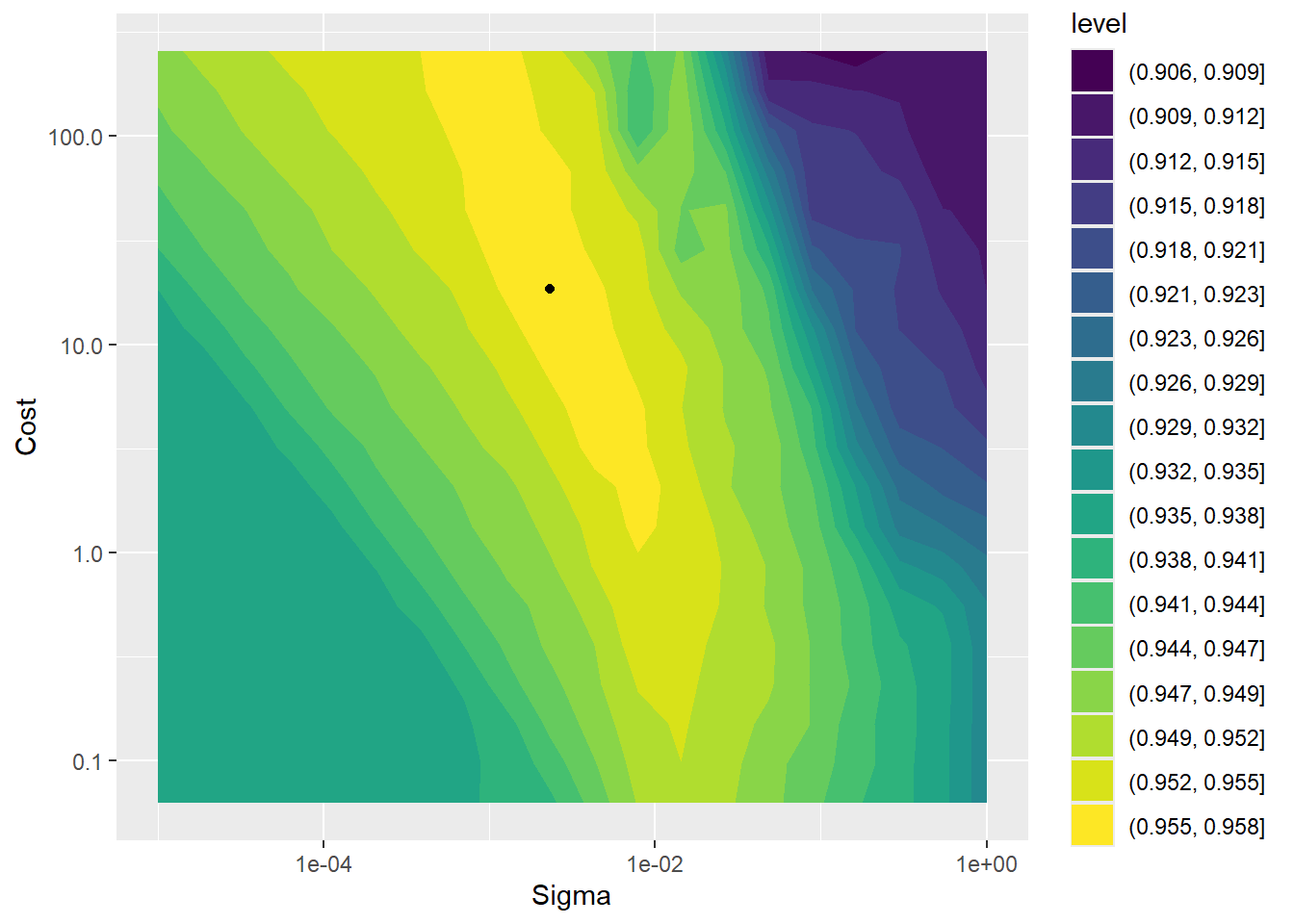
The plot above shows the model’s performance (mean ROC_AUC value over the 5 folds) as function of the hyperparameters cost and sigma. The plotted point shows the value with the highest performance.
Note that if you tuned the hyperparameters on a coarser grid, then the plot will be different (coarser).
9 Final fit and predictions
Using the tuned hyperparameters (thus the best combination of hyperparameters in terms of performance on the validation datasets), we can now proceed to the last step in a predictive machine learning pipeline After having established the best values of the hyperparameters, we need to:
- update the specification of the model (by filling in the tuned values of the hyperparameters);
- train the data recipe on the entire model development
dataset (thus:
prepthe data recipe on the entiretrainingpart of themain_splitdata split); - bake the training, as well as the testing data, using the prepared data recipe;
- fit the updated model to the prepared training data;
- predict the fitted model onto the prepared testing data;
- evaluate the predictive performance of the fitted model on the testing data.
We could do these steps by repeating the steps done above (i.e. exercises 13.3 - 13.7) with an updated specification of the model and an updated definition of the training and testing data (thus: not the k cross validation folds, but the main train-test data split).
Alternatively, and more efficiently, we could use several dedicated tidymodels functions to do this:
- function
select_bestselects the best combination of hyperparameters from a tuned grid (here from the objectsvm_resthat holds the results of thetune_gridfunction) based on a specified metric that will be used to sort the models in the grid (e.g., based on the metric “roc_auc”); - function
finalize_modelcan be used to then update a model specification with the selected hyperparameters (as done in the previous step); - function
update_modelcan then be used to update the model specification in an existing workflow object: it first removes the existing model specification and then adds the new specification to the workflow; - function
last_fitcan then be used to perform the final model fit on the entire training set (e.g. the entire dataset that was used during cross-validation) and then predicts the fitted model using the left out test dataset (that was not used in any of the steps above during model development!). This last step will thus quantify the predictive performance of the model! The model predictions and prediction metrics can then be retrieved using thecollect_metricsandcollect_predictionsfunctions.
For example, the following sequence of operations, with hypothetical names for the different types of objects (e.g. for the hyperparameter tuning results, the model specification, the specified workflow and the specification of a train-test datasplit) will combine all these steps:
# Get best hyperparameter values based on ROC-AUC
best_hyperparms <- tuning_results %>%
  select_best(metric = "roc_auc")

# Update the model-specification using these best hyperparameters
final_model <- model_specification %>%
  finalize_model(best_hyperparms)

# Update the workflow
model_workflow_final <- model_workflow %>%
  update_model(final_model)

# check the steps above
model_workflow_final

# perform a last fit of the model
# based on ALL training data
# and predict on the TESTING data
final_fit <- model_workflow_final %>%
  last_fit(train_test_split)

# Inspect result
final_fit

# collect metrics
final_fit %>%
  collect_metrics()

# get predictions
final_fit %>%
  collect_predictions() %>%
  conf_mat(truth = isGrazing,
           estimate = .pred_class)
Exercise 13.9a
Using the different objects created in the exercises above, select the
best combination of hyperparameters according to ROC-AUC, update the
model specification and workflow, refit the model on the entire model
development dataset (thus, the training part of the
main_split object) and assess its predictive performance on
the testing dataset (show both the prediction metrics, ass well
as the confusion matrix). # Get best hyperparameter values based on ROC-AUC
best_auc <- svm_res %>%
select_best(metric = "roc_auc")
# Update the model-specification using these best hyperparameters
final_model <- svm_spec %>%
finalize_model(best_auc)
# Update the workflow
svm_wf_final <- svm_wf %>%
update_model(final_model)
# Inspect result
svm_wf_final## ══ Workflow ════════════════════════════════════════════════════════════════════════════════════════════════════════════════════════════════════════════════════════
## Preprocessor: Recipe
## Model: svm_rbf()
##
## ── Preprocessor ────────────────────────────────────────────────────────────────────────────────────────────────────────────────────────────────────────────────────
## 3 Recipe Steps
##
## • step_rm()
## • step_center()
## • step_scale()
##
## ── Model ───────────────────────────────────────────────────────────────────────────────────────────────────────────────────────────────────────────────────────────
## Radial Basis Function Support Vector Machine Model Specification (classification)
##
## Main Arguments:
## cost = 16
## rbf_sigma = 0.00599484250318941
##
## Computational engine: kernlab# perform a last fit of the model based on ALL the training data, and predict on the TESTING data
svm_wf_final_fit <- svm_wf_final %>%
last_fit(main_split)
# collect metrics
svm_wf_final_fit %>%
collect_metrics()## # A tibble: 3 × 4
## .metric .estimator .estimate .config
## <chr> <chr> <dbl> <chr>
## 1 accuracy binary 0.936 pre0_mod0_post0
## 2 roc_auc binary 0.958 pre0_mod0_post0
## 3 brier_class binary 0.0504 pre0_mod0_post0# get predictions
svm_wf_final_fit %>%
collect_predictions() %>%
conf_mat(truth = isGrazing,
estimate = .pred_class)## Truth
## Prediction FALSE TRUE
## FALSE 85 21
## TRUE 18 484The selected best hyperparameters are: cost = 16 and rbf_sigma = 0.00599. The model fits the test data very well: the overall accuracy of prediction is 93.6%!
10 Challenge
Challenge
Above we only have focussed on a kernel SVM using the “kernlab”
implementation as the engine. As a challenge, try using a different
algorithm, e.g. a neural network (e.g. in the “nnet” or “keras”
implementation, or a random forest (e.g. in the “randomForest” or
“ranger” implementation). See
here
for examples. You can focus on mlp for neural networks (a
multilayer perceptron model a.k.a. a single layer, feed-forward neural
network) or rand_forest for random forests,
respectively.
A random forest could be fitted and tuned as follows;
# Load library for engine
library(ranger)

# Specify model
rf_spec <- rand_forest(trees = 1000,
                       mtry = tune(),
                       min_n = tune(),
                       mode = "classification") %>%
  set_engine("ranger", seed = 1234567)

# Bundle specification of data recipe and model into workflow
rf_wf <- workflow() %>%
  add_model(rf_spec) %>%
  add_recipe(dat_rec)

# Specify grid of hyperparameter values for which to assess fit
rf_grid <- grid_regular(mtry(range = c(1,5)),
                        min_n(range = c(1,10)),
                        levels = 10)

# Tune the hyperparameters with the elements prepared above
rf_res <- rf_wf %>%
  tune_grid(resamples = dat_split,
            grid = rf_grid)

# Get best hyperparameter values based on ROC-AUC
rf_best <- rf_res %>%
  select_best(metric = "roc_auc")

# Update the model-specification using these best hyperparameters
rf_final <- rf_spec %>%
  finalize_model(rf_best)

# Update the workflow
rf_wf_final <- rf_wf %>%
  update_model(rf_final)

# check the steps above
rf_wf_final

# perform a last fit of the model
# based on ALL training data
# and predict on the TESTING data
rf_final_fit <- rf_wf_final %>%
  last_fit(main_split)

# Inspect result
rf_final_fit

# collect metrics
rf_final_fit %>%
  collect_metrics()

# get predictions
rf_final_fit %>%
  collect_predictions() %>%
  conf_mat(truth = isGrazing,
           estimate = .pred_class)
Tuning and fitting a neural network using Keras could be done using:
# Load library for engine
library(nnet)

# Specify model
nn_spec <- mlp(hidden_units = tune(),
               penalty = tune(),
               dropout = 0.0,
               epochs = 20,
               activation = "softmax") %>%
  set_engine("nnet", seed = 1234567) %>%
  set_mode("classification")

# Bundle specification of data recipe and model into workflow
nn_wf <- workflow() %>%
  add_model(nn_spec) %>%
  add_recipe(dat_rec)

# Specify grid of hyperparameter values for which to assess fit
nn_grid <- grid_regular(hidden_units(range = c(1,10)),
                        penalty(range = c(-10,0)),
                        levels = 10)

# Tune the hyperparameters with the elements prepared above
nn_res <- nn_wf %>%
  tune_grid(resamples = dat_split,
            grid = nn_grid)

# Get best hyperparameter values based on ROC-AUC
nn_best <- nn_res %>%
  select_best(metric = "roc_auc")

# Update the model-specification using these best hyperparameters
nn_final <- nn_spec %>%
  finalize_model(nn_best)

# Update the workflow
nn_wf_final <- nn_wf %>%
  update_model(nn_final)

# check the steps above
nn_wf_final

# perform a last fit of the model
# based on ALL training data
# and predict on the TESTING data
nn_final_fit <- nn_wf_final %>%
  last_fit(main_split)

# Inspect result
nn_final_fit

# collect metrics
nn_final_fit %>%
  collect_metrics()

# get predictions
nn_final_fit %>%
  collect_predictions() %>%
  conf_mat(truth = isGrazing,
           estimate = .pred_class)
11 Submit your last plot
Submit your script file as well as a plot: either your last created plot, or a plot that best captures your solution to the challenge. Submit the files on Brightspace via Assessment > Assignments > Skills day 13.
Note that your submission will not be graded or evaluated. It is used only to facilitate interaction and to get insight into progress.
11 Recap
Today, we’ve further explored the tidymodels packages, including the workflows, dials and tune packages that we used to perform hyperparameter tuning.
An R script of today’s exercises can be downloaded here