Use the function unite in the tidyr package to
paste columns together. Use the str_replace or
str_replace_all function (form the stringr
package, part of core tidyverse) to replace specific patterns from a
string with a replacement pattern.
Tidying data using tidyr
Overview
Today’s goal: to be able to transform datasets into a tidy format using the tidyr package
Resources
- R4DS: chapters 12 tidy data
- tidy data
Packages
Main functions
pivot_longer, pivot_wider, separate_wider_delim, unite, complete.
Cheat sheets
In this tutorial, we will practice putting data into a tidy format using the package tidyr, and also use some handy data cleaning and preparation tools from the stringr package.
Remember, properties of a tidy dataset are:
- Each variable is in its own column;
- Each case/observation is in its own row.
1 Phenology data
To practice data tidying, we will use the data from the Chronicles of Nature dataset, as made publicly available in Ovaskainen et al. 2020. We will be using this extensive, large-scale, long-term and multi-taxon database on phenological and climatic variation to reproduce some figures shown in Ovaskainen et al. 2013 about the community-level phenological response of several species to climate change.
The full dataset consist of more than half a million records from 471 localities in the Russian Federation, Ukraine, Uzbekistan, Belarus and Kyrgyzstan, in which nature reserves recorded the timing of specified climatic and phenological events. The data go back to as early as 1890, but most data is post 1960. We will look at some trends in phenological events for a single site, Kivach, during 40 years.
Exercise 6.1a
Download the file chroniclesofnature.csv from Brightspace
> Skills > Datasets > Phenology. Remember to save it at
the appropriate place, for example, put the data in the folder
data/raw/phenology/. Load the downloaded csv file into a
tibble called dat. # Prelims
library(tidyverse)
# setwd()
# Load data
dat <- read_csv("data/raw/phenology/chroniclesofnature.csv")2 Tidy the data
The data are not yet in tidy format. Here, we are going to tidy the data by transforming it so that each row/record corresponds to a year in which data is gathered, each column corresponds to a feature (i.e., a climatic or phenological event), and each value in the feature columns correspond to the timing of the event in terms of day-of-year. The data consists of the following columns:
- taxon: the climatological measure, or species name (values: Temperature, Scolopax rusticola, Bombus, Tussilago farfara, Salix caprea, Zootoca vivipara);
- event: the event that was registered (values: transition above 0, start of display flights, 1st occurrence, onset of blooming);
- year: year, e.g., 1970;
- dayofyear: the day of the year on which the event took place, e.g., 150.
Exercise 6.2a
Unite the columns taxon and event into a single column
called event, separated by an underscore, _. Also
replace the spaces in the newly created column by a dot, ..
dat <- dat %>%
  unite(col = "event", taxon:event, sep = "_") %>%
  mutate(event = str_replace_all(event,
                                 pattern=" ",
                                 replacement="."))
dat
## # A tibble: 246 × 3
## event year dayofyear
## <chr> <dbl> <dbl>
## 1 Temperature_transition.above.0 1966 112
## 2 Temperature_transition.above.0 1967 86
## 3 Temperature_transition.above.0 1968 82
## 4 Temperature_transition.above.0 1969 99
## 5 Temperature_transition.above.0 1970 92
## 6 Temperature_transition.above.0 1971 121
## 7 Temperature_transition.above.0 1972 98
## 8 Temperature_transition.above.0 1973 83
## 9 Temperature_transition.above.0 1974 117
## 10 Temperature_transition.above.0 1975 64
## # ℹ 236 more rows
Exercise 6.2b
In the csv file loaded above, we’ve removed a few years of data. Which
years? Update object dat so that these years are also
included, with value NA. First, to check for a sorted series of unique values, you can make
use of the sort and unique functions.
Functions like summary, range,
min and max can be used to retrieve basic
summaries of numeric data (here e.g. start and end year of sampling). To
get values that are not present in a vector you could make use of the
! and %in% operators, especially in
combination with square bracket indexing, e.g. the following code checks
which values in x do not occur in y:
x <- 1:6
y <- c(1, 2, 4, 5)
x[! x %in% y]
## [1] 3 6Then, you can use the complete function to complete a
tibble with missing combinations of data.
When you have completed the dataset, you should have 288 records.
sort(unique(dat$year))## [1] 1966 1967 1968 1969 1970 1971 1972 1973 1974 1975 1976 1977 1978 1979 1980 1981 1982 1983 1984 1985 1986 1987 1988 1989 1990 1994 1995 1996 1997 1998 1999 2000
## [33] 2001 2002 2003 2004 2005 2006 2007 2008 2009 2010 2011 2012 2013range(dat$year) # 1966 - 2013## [1] 1966 2013allyears = seq.int(from = 1966, to = 2013)
allyears[! allyears %in% dat$year]## [1] 1991 1992 1993Thus, the years 1991:1993 are missing: this was the time of the Soviet breakup. Now, we can compete the dataset using all years:
dat <- dat %>%
  complete(year = allyears, event)
dat %>%
  filter(year %in% c(1991:1993))
## # A tibble: 18 × 3
## year event dayofyear
## <dbl> <chr> <dbl>
## 1 1991 Bombus_1st.occurrence NA
## 2 1991 Salix.caprea_onset.of.blooming NA
## 3 1991 Scolopax.rusticola_start.of.display.flights NA
## 4 1991 Temperature_transition.above.0 NA
## 5 1991 Tussilago.farfara_onset.of.blooming NA
## 6 1991 Zootoca.vivipara_1st.occurrence NA
## 7 1992 Bombus_1st.occurrence NA
## 8 1992 Salix.caprea_onset.of.blooming NA
## 9 1992 Scolopax.rusticola_start.of.display.flights NA
## 10 1992 Temperature_transition.above.0 NA
## 11 1992 Tussilago.farfara_onset.of.blooming NA
## 12 1992 Zootoca.vivipara_1st.occurrence NA
## 13 1993 Bombus_1st.occurrence NA
## 14 1993 Salix.caprea_onset.of.blooming NA
## 15 1993 Scolopax.rusticola_start.of.display.flights NA
## 16 1993 Temperature_transition.above.0 NA
## 17 1993 Tussilago.farfara_onset.of.blooming NA
## 18 1993 Zootoca.vivipara_1st.occurrence NA
Exercise 6.2c
Check how many rows and columns the object dat contains.
Transform the tibble into wider format, by transforming each distinct
value in the event column to a new column, filled with values
found in dayofyear. Assign the result to a new object called
dat2. Check the number of rows and columns in this tibble.
Use the pivot_wider function.
nrow(dat); ncol(dat)## [1] 288## [1] 3dat2 <- dat %>%
pivot_wider(names_from = event,
values_from = dayofyear)
nrow(dat2); ncol(dat2)## [1] 48## [1] 7The tibble dat has 288 rows and 3 columns (thus: a
‘long’ format), while the tibble dat2 has 48 rows and 7
columns (thus a ‘wide’ format - hence the function name
pivot_wider).
Exercise 6.2d
Recreate figure 2a in
Ovaskainen
et al. 2013: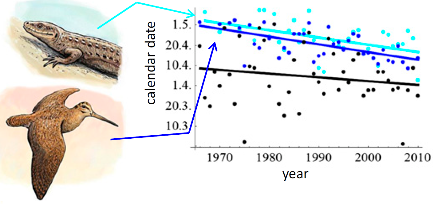
Note that you can simply plot the day of year of the phenological event on the y axis: you do not have to convert it to a date.
dat2 %>%
  ggplot() +

  geom_point(aes(x=year,
                 y=Temperature_transition.above.0),
             col="black") +
  geom_smooth(aes(x=year,
                  y=Temperature_transition.above.0),
              method="lm", se=FALSE, col="black") +

  geom_point(aes(x=year,
                 y=Scolopax.rusticola_start.of.display.flights),
             col="blue") +
  geom_smooth(aes(x=year,
                  y=Scolopax.rusticola_start.of.display.flights),
              method="lm", se=FALSE, col="blue") +

  geom_point(aes(x=year,
                 y=Zootoca.vivipara_1st.occurrence),
             col="cyan") +
  geom_smooth(aes(x=year,
                  y=Zootoca.vivipara_1st.occurrence),
              method="lm", se=FALSE, col="cyan") +

  xlab("Year") +
  ylab("Day of year") +
  ggtitle("Phenological shift")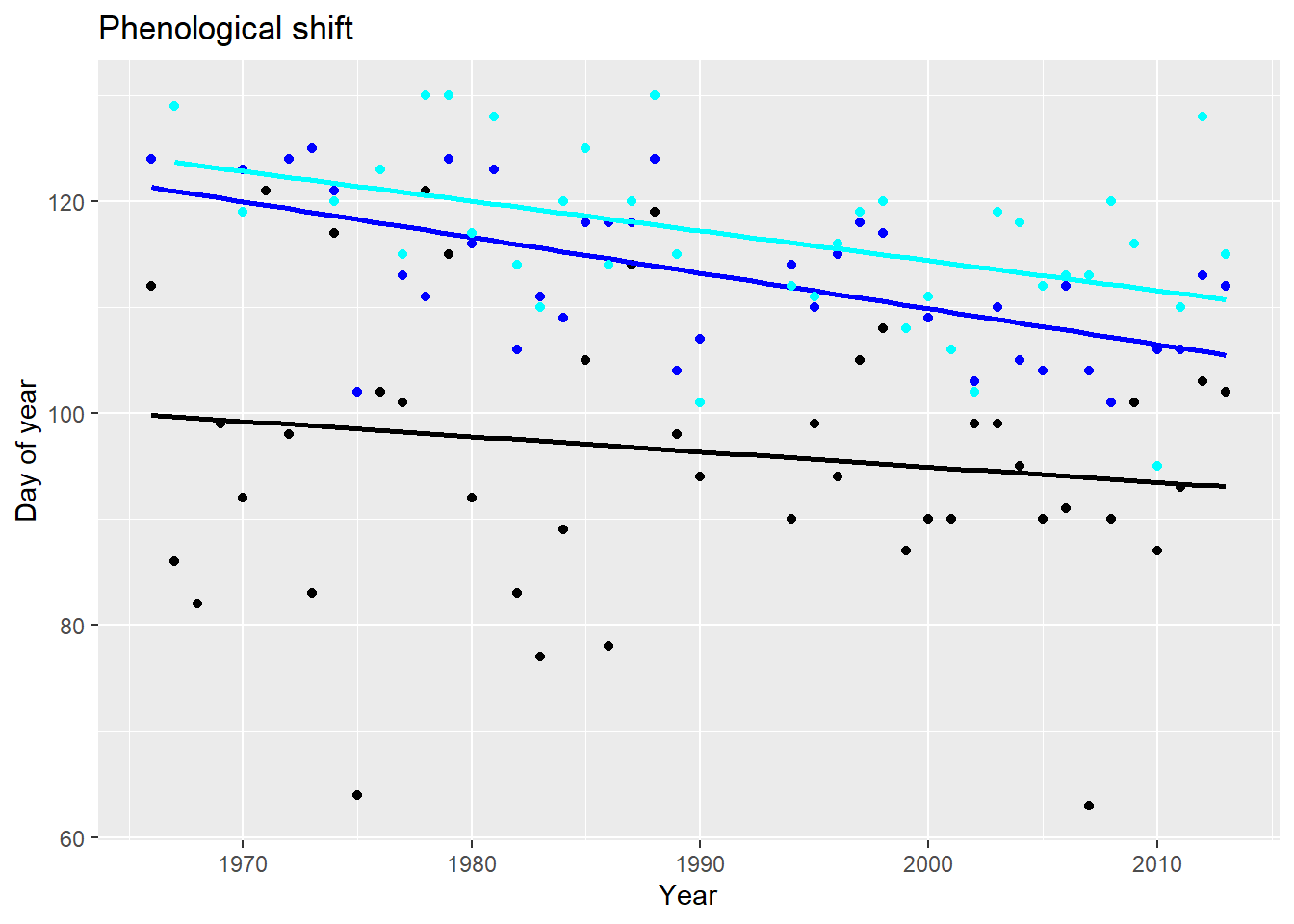
Exercise 6.2e
Recreate figure 4a in
Ovaskainen
et al. 2013: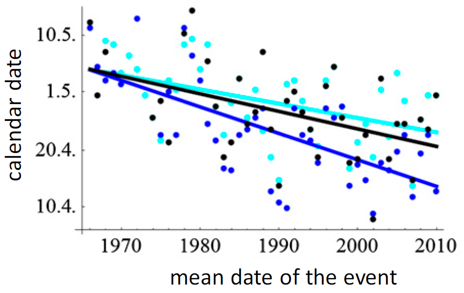
Note that you can simply plot the day of year of the phenological event on the y axis: you do not have to convert it to a date.
dat2 %>%
  ggplot() +

  geom_point(aes(x=year,
                 y=Bombus_1st.occurrence),
             col="black") +
  geom_smooth(aes(x=year,
                  y=Bombus_1st.occurrence),
              method="lm", se=FALSE, col="black") +

  geom_point(aes(x=year,
                 y=Salix.caprea_onset.of.blooming),
             col="cyan") +
  geom_smooth(aes(x=year,
                  y=Salix.caprea_onset.of.blooming),
              method="lm", se=FALSE, col="cyan") +

  geom_point(aes(x=year,
                 y=Tussilago.farfara_onset.of.blooming), col="blue") +
  geom_smooth(aes(x=year,
                  y=Tussilago.farfara_onset.of.blooming),
              method="lm", se=FALSE, col="blue") +

  xlab("Year") +
  ylab("Day of year") +
  ggtitle("Phenological shift")
Exercise 6.2f
Create a new plot showing blooming of species as function of temperature
transition above 0. dat2 %>%
ggplot(aes(x=Temperature_transition.above.0)) +
geom_point(aes(y=Salix.caprea_onset.of.blooming),
col="red") +
geom_smooth(aes(y=Salix.caprea_onset.of.blooming),
method="lm", se=FALSE, col="red") +
geom_point(aes(y=Tussilago.farfara_onset.of.blooming),
col="blue") +
geom_smooth(aes(y=Tussilago.farfara_onset.of.blooming),
method="lm", se=FALSE, col="blue") +
xlab("Temperature transition above 0") +
ylab("Day of blooming") +
ggtitle("Phenological shift")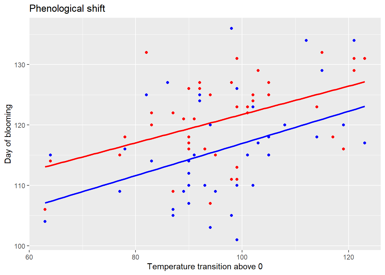
Exercise 6.2g
Convert the dataset back to long format and assign it to an
object called dat3. Assign the names to the new column
feature, and the values to new column with name
dayofyear. How many rows do you have and how does this
compare to the original data? Use the pivot_longer function.
dat3 <- dat2 %>%
  pivot_longer(2:7,
               names_to = "feature",
               values_to = "dayofyear",
               values_drop_na = FALSE)
nrow(dat3)
## [1] 288nrow(dat)## [1] 288Now we have 288 rows, and this is the same as the number of rows in
the original tibble dat.
Exercise 6.2h
Separate the column feature into the columns taxon and
event, based on a split of its contents on the underscore
symbol. Afterwards, you can replace the dots back to spaces. Use the separate_wider_delim function from the tidyr
package. Note that if there are strings with multiple underscore
symbols, you can instruct the separate_wider_delim function
how to deal with this situation; see the function documentation,
especially the function argument too_many.
Use the str_replace or str_replace_all
function to replace specific patterns from a string with a replacement
pattern. Note that the pattern to be replaced can be a
regular expression, see the function help file; using
pattern = "." might not work, in which case you could use
`pattern = “[.]” or one of the other methods.
dat3 <- dat3 %>%
  separate_wider_delim(
    feature,
    names = c("taxon","event"),
    delim = '_',
    too_many = "merge",
    cols_remove = TRUE) %>%
  mutate(
    taxon = str_replace_all(taxon,
                            pattern = "[.]",
                            replacement = " "),
    event = str_replace_all(event,
                            pattern = "[.]",
                            replacement = " "))
dat3
## # A tibble: 288 × 4
## year taxon event dayofyear
## <dbl> <chr> <chr> <dbl>
## 1 1966 Bombus 1st occurrence 135
## 2 1966 Salix caprea onset of blooming NA
## 3 1966 Scolopax rusticola start of display flights 124
## 4 1966 Temperature transition above 0 112
## 5 1966 Tussilago farfara onset of blooming 134
## 6 1966 Zootoca vivipara 1st occurrence NA
## 7 1967 Bombus 1st occurrence 122
## 8 1967 Salix caprea onset of blooming NA
## 9 1967 Scolopax rusticola start of display flights NA
## 10 1967 Temperature transition above 0 86
## # ℹ 278 more rows3 Challenge
Challenge - tidying the COVID-19 data
In this challenge, you are going to load and tidy an online dataset on COVID cases across countries. We can access the John Hopkins university global dataset of numbers of confirmed COVID cases directly from a csv file on github:
"https://raw.githubusercontent.com/CSSEGISandData/COVID-19/master/csse_covid_19_data/csse_covid_19_time_series/time_series_covid19_confirmed_global.csv"Load this dataset into R using the appropriate tidyverse functions.
Then, remove the columns “Province/State”, “Lat” and “Long”, and rename the column “Country/Region” to “country”. Check the number of rows and columns that the dataset contains. In this dataset, each date has its own column, thus this dataset is not tidy yet. Therefore, make it a tidy dataset, where each record is a row, each feature a column. After tidying, how many rows and columns does the dataset have?The function matches can find column names that match a
specific expression, where “\d” is the expression for a any numeric
character. Note that because this pattern contains a back-slash, it
needs to be ‘escaped’. In R, you can escape a special character by
putting a back-slack in front of it, here thus “\\d”.
# load data
confirmedraw <- read_csv("https://raw.githubusercontent.com/CSSEGISandData/COVID-19/master/csse_covid_19_data/csse_covid_19_time_series/time_series_covid19_confirmed_global.csv")

# Inspect
confirmedraw
## # A tibble: 289 × 1,147
## `Province/State` `Country/Region` Lat Long `1/22/20` `1/23/20` `1/24/20` `1/25/20` `1/26/20` `1/27/20` `1/28/20` `1/29/20` `1/30/20` `1/31/20` `2/1/20`
## <chr> <chr> <dbl> <dbl> <dbl> <dbl> <dbl> <dbl> <dbl> <dbl> <dbl> <dbl> <dbl> <dbl> <dbl>
## 1 <NA> Afghanistan 33.9 67.7 0 0 0 0 0 0 0 0 0 0 0
## 2 <NA> Albania 41.2 20.2 0 0 0 0 0 0 0 0 0 0 0
## 3 <NA> Algeria 28.0 1.66 0 0 0 0 0 0 0 0 0 0 0
## 4 <NA> Andorra 42.5 1.52 0 0 0 0 0 0 0 0 0 0 0
## 5 <NA> Angola -11.2 17.9 0 0 0 0 0 0 0 0 0 0 0
## 6 <NA> Antarctica -71.9 23.3 0 0 0 0 0 0 0 0 0 0 0
## 7 <NA> Antigua and Bar… 17.1 -61.8 0 0 0 0 0 0 0 0 0 0 0
## 8 <NA> Argentina -38.4 -63.6 0 0 0 0 0 0 0 0 0 0 0
## 9 <NA> Armenia 40.1 45.0 0 0 0 0 0 0 0 0 0 0 0
## 10 Australian Capital Te… Australia -35.5 149. 0 0 0 0 0 0 0 0 0 0 0
## # ℹ 279 more rows
## # ℹ 1,132 more variables: `2/2/20` <dbl>, `2/3/20` <dbl>, `2/4/20` <dbl>, `2/5/20` <dbl>, `2/6/20` <dbl>, `2/7/20` <dbl>, `2/8/20` <dbl>, `2/9/20` <dbl>,
## # `2/10/20` <dbl>, `2/11/20` <dbl>, `2/12/20` <dbl>, `2/13/20` <dbl>, `2/14/20` <dbl>, `2/15/20` <dbl>, `2/16/20` <dbl>, `2/17/20` <dbl>, `2/18/20` <dbl>,
## # `2/19/20` <dbl>, `2/20/20` <dbl>, `2/21/20` <dbl>, `2/22/20` <dbl>, `2/23/20` <dbl>, `2/24/20` <dbl>, `2/25/20` <dbl>, `2/26/20` <dbl>, `2/27/20` <dbl>,
## # `2/28/20` <dbl>, `2/29/20` <dbl>, `3/1/20` <dbl>, `3/2/20` <dbl>, `3/3/20` <dbl>, `3/4/20` <dbl>, `3/5/20` <dbl>, `3/6/20` <dbl>, `3/7/20` <dbl>,
## # `3/8/20` <dbl>, `3/9/20` <dbl>, `3/10/20` <dbl>, `3/11/20` <dbl>, `3/12/20` <dbl>, `3/13/20` <dbl>, `3/14/20` <dbl>, `3/15/20` <dbl>, `3/16/20` <dbl>,
## # `3/17/20` <dbl>, `3/18/20` <dbl>, `3/19/20` <dbl>, `3/20/20` <dbl>, `3/21/20` <dbl>, `3/22/20` <dbl>, `3/23/20` <dbl>, `3/24/20` <dbl>, `3/25/20` <dbl>, …# tidy
confirmed <- confirmedraw %>%
select(-"Province/State", -Lat, -Long) %>%
rename(country = "Country/Region") %>%
pivot_longer(cols = matches("\\d/."),
names_to = "date",
values_to = "confirmed")
# inspect
confirmed## # A tibble: 330,327 × 3
## country date confirmed
## <chr> <chr> <dbl>
## 1 Afghanistan 1/22/20 0
## 2 Afghanistan 1/23/20 0
## 3 Afghanistan 1/24/20 0
## 4 Afghanistan 1/25/20 0
## 5 Afghanistan 1/26/20 0
## 6 Afghanistan 1/27/20 0
## 7 Afghanistan 1/28/20 0
## 8 Afghanistan 1/29/20 0
## 9 Afghanistan 1/30/20 0
## 10 Afghanistan 1/31/20 0
## # ℹ 330,317 more rowsdim(confirmedraw)## [1] 289 1147dim(confirmed)## [1] 330327 3Optionally, we can now plot it:
library(lubridate) # tidyverse package to work with date/time data
confirmed_dense <- confirmed %>%
  mutate(confirmed = as.integer(confirmed),
         date = mdy(date)) %>%
  filter(confirmed > 0) %>%
  group_by(country,date) %>%
  summarize(total = sum(confirmed)) %>%
  arrange(country,date, total)

confirmed_dense %>%
  ggplot(aes(x=date, y=total, colour=country)) +
  geom_line() +
  theme(legend.position = "none") +
  labs(title = "Coronavirus trajectories for 192 countries ",
       subtitle = "Cumulative number of cases according to the John Hopkins database",
       x = "Date",
       y = NULL) +
  scale_y_log10(name = "Confirmed cases",
                limits = c(1, 100000000),
                breaks = c(1, 10, 100, 1000, 10000, 100000,1000000,10000000),
                labels = c("1", "10", "100", "1,000", "10,000", "100,000","1,000,000", "10,000,000"),
                sec.axis = dup_axis()) +
  annotation_logticks(sides = "lr") +
  theme_bw() +
  theme(plot.background = element_rect(fill = rgb(255,241,230,max=255)),
        panel.background = element_rect(fill = rgb(255,241,230,max=255)),
        legend.position="none",
        panel.grid.major = element_line(colour = "grey"))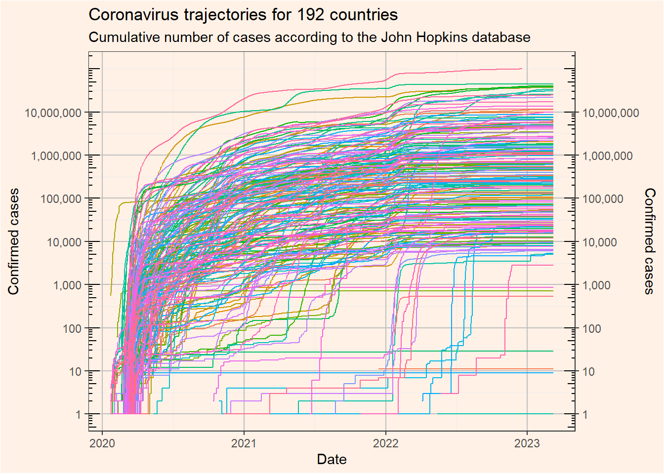
4 Submit your last plot
Submit your script file as well as a plot: either your last created plot, or a plot that best captures your solution to the challenge. Submit the files on Brightspace via Assessment > Assignments > Skills day 6.
Note that your submission will not be graded or evaluated. It is used only to facilitate interaction and to get insight into progress.
5 Recap
Today, we’ve explored methods to get untidy data into a tidy form, using the tidyr package. Tomorrow, we will explore a set of tools to efficiently work with character strings, timestamps, write our own functions, and explore methods for iteration.
An R script of today’s exercises can be downloaded here
6 Further reading
Further reading