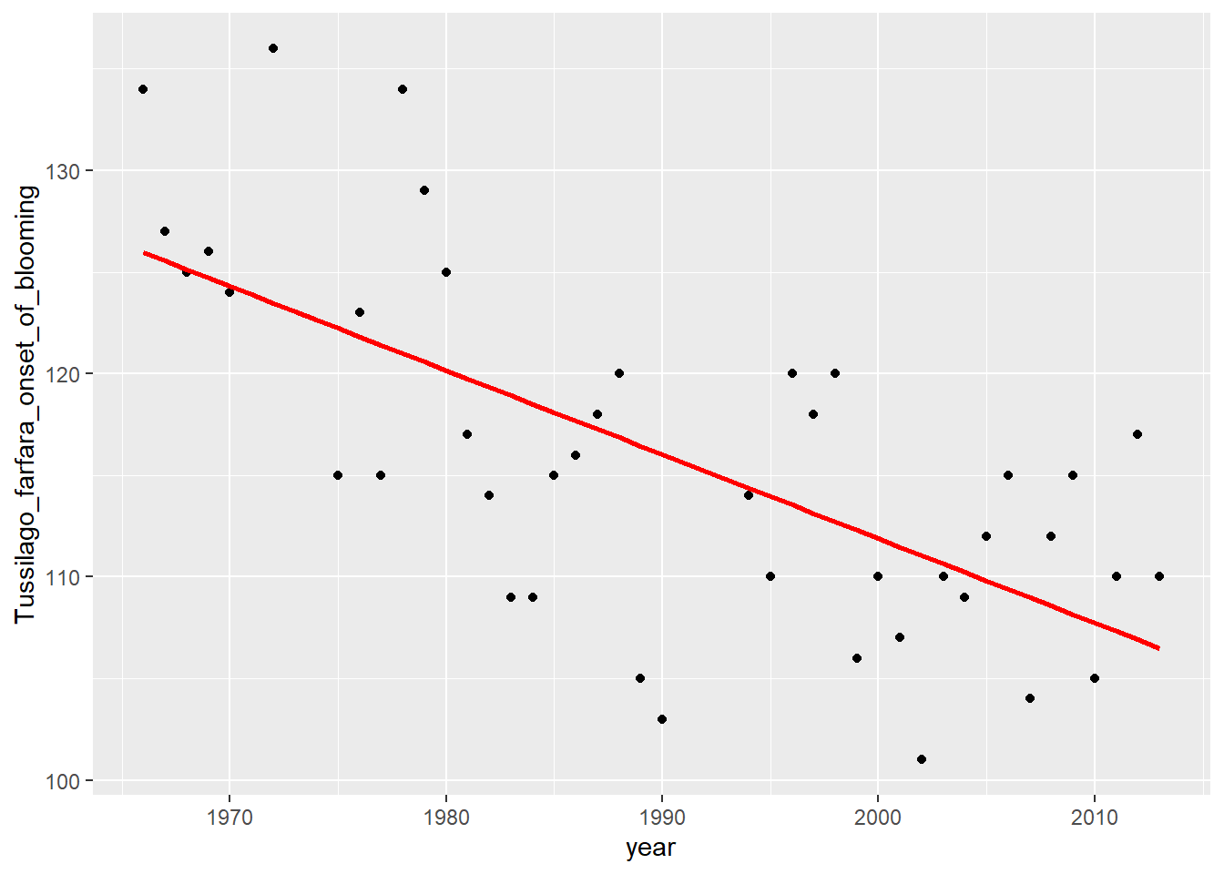
In Monday’s exercises, we studied the synchrony between phenological
events of pollinators (e.g. the first appearance of bumblebees,
Bombus spp.) and plants (e.g. the onset of blooming in goat
willows, Salix caprea, and coltsfoot, Tussilago
farfara), using long-term data collected across many locations in
the Russian Federation, Ukraine, Uzbekistan, Belarus and Kyrgyzstan (see
Ovaskainen
et al. 2013). In Exercise 6.2e we saw that the first occurrence of
bumblebees has a higher level of synchrony with the onset of flowering
of goat willows than that of coltsfoot. This may suggest that in these
areas, the blooming of the goat willow might represent the basic source
of food for bumblebees in the first days after their emergence in early
spring. Thus, the results from Monday’s analyses might suggest that the
appearance of bumblebees has shifted in parallel with the blossoming of
goat willow, whereas the blooming of coltsfoot has shifted faster.
In this challenge, let’s thus model the synchrony between the first
appearance of bumblebees and the blooming onset of goat willows
further:
# Prepare data and fit models per study site
datmodels <- dat %>%
  # keep only relevant columns
  select(year,
         studysite,
         Bombus_1st_occurrence,
         Salix_caprea_onset_of_blooming) %>%
  # drop rows on with NAs
  drop_na() %>%
  # nest data per study site
  nest(.by = studysite) %>%
  # get nr records per study site
  mutate(n = map_int(data, nrow)) %>%
  # Keep only study areas with 10 records or more
  filter(n >= 10) %>%
  mutate(
    # Fit models
    lmfit = map(data,
                .f = function(x){
                  lm(Bombus_1st_occurrence ~ Salix_caprea_onset_of_blooming, data = x)
                }),
    # get beta coefficient for the slope
    slope = map_dbl(lmfit,
                    .f = function(x){
                      coefficients(x)[2]
                    }),
    # get r2 values for the model fits
    r2 = map_dbl(lmfit,
                 .f = function(x){
                   summary(x)$r.squared
                 })
  )

# Explore data
datmodels
## # A tibble: 18 × 6
##    studysite                         data                  n lmfit    slope       r2
##    <chr>                             <list>            <int> <list>   <dbl>    <dbl>
##  1 Nikel (Murmansk)                  <tibble [11 × 3]>    11 <lm>    0.915  0.586
##  2 Laplandskij                       <tibble [60 × 3]>    60 <lm>    0.593  0.370
##  3 Pechoro-Ilychskij                 <tibble [62 × 3]>    62 <lm>    0.742  0.441
##  4 Prioksko-Terrasnyj                <tibble [32 × 3]>    32 <lm>    0.0215 0.000586
##  5 Pinega (Arkhangelsk)              <tibble [19 × 3]>    19 <lm>    0.705  0.439
##  6 Kirovsk (Murmansk)                <tibble [12 × 3]>    12 <lm>   -0.0632 0.0125
##  7 Georgiyevskoye (Arkhangelsk)      <tibble [18 × 3]>    18 <lm>    0.874  0.577
##  8 Kurtsevo (Arkhangelsk)            <tibble [21 × 3]>    21 <lm>    1.37   0.542
##  9 Kivach                            <tibble [36 × 3]>    36 <lm>    0.829  0.422
## 10 Manushkino-Nyandoma (Arkhangelsk) <tibble [31 × 3]>    31 <lm>    0.815  0.427
## 11 Mezen (Arkhangelsk)               <tibble [10 × 3]>    10 <lm>    0.981  0.700
## 12 Altajskij_Yailu                   <tibble [18 × 3]>    18 <lm>    0.731  0.432
## 13 Konevo (Arkhangelsk)              <tibble [15 × 3]>    15 <lm>    0.843  0.420
## 14 Kargopol (Arkhangelsk)            <tibble [11 × 3]>    11 <lm>    0.745  0.321
## 15 Pinezhskij                        <tibble [33 × 3]>    33 <lm>    0.603  0.627
## 16 Kostomukshskij                    <tibble [23 × 3]>    23 <lm>    0.277  0.0960
## 17 Kenozerskij                       <tibble [10 × 3]>    10 <lm>    0.950  0.369
## 18 Altajskij_Bele                    <tibble [12 × 3]>    12 <lm>    0.150  0.0143
# Plot
datmodels %>%
  select(studysite, data, slope, r2) %>%
  unnest(data) %>%
  mutate(r2_class =
           case_when(r2 <= 0.2 ~ "a", # or, use function cut()
                     r2 > 0.2 & r2 <= 0.5 ~ "b",
                     r2 > 0.5 ~ "c"),
         r2_class = factor(r2_class,
                           levels = c("a","b","c"),
                           labels = c("r2 <= 0.2",
                                      "0.2 < r2 <= 0.5",
                                      "r2 > 0.5"))) %>%
  ggplot(mapping = aes(x = Salix_caprea_onset_of_blooming,
                       y = Bombus_1st_occurrence,
                       col = studysite)) +
  geom_point() +
  geom_smooth(method = "lm") +
  geom_abline(intercept = 0, slope = 1, # dashed line with 1:1 relationship
              col = "black", linetype = "dashed") +
  labs(x = "Salix caprea onset of blooming",
       y = "Bombus 1st occurrence",
       col = "Study area") +
  facet_wrap(~r2_class)
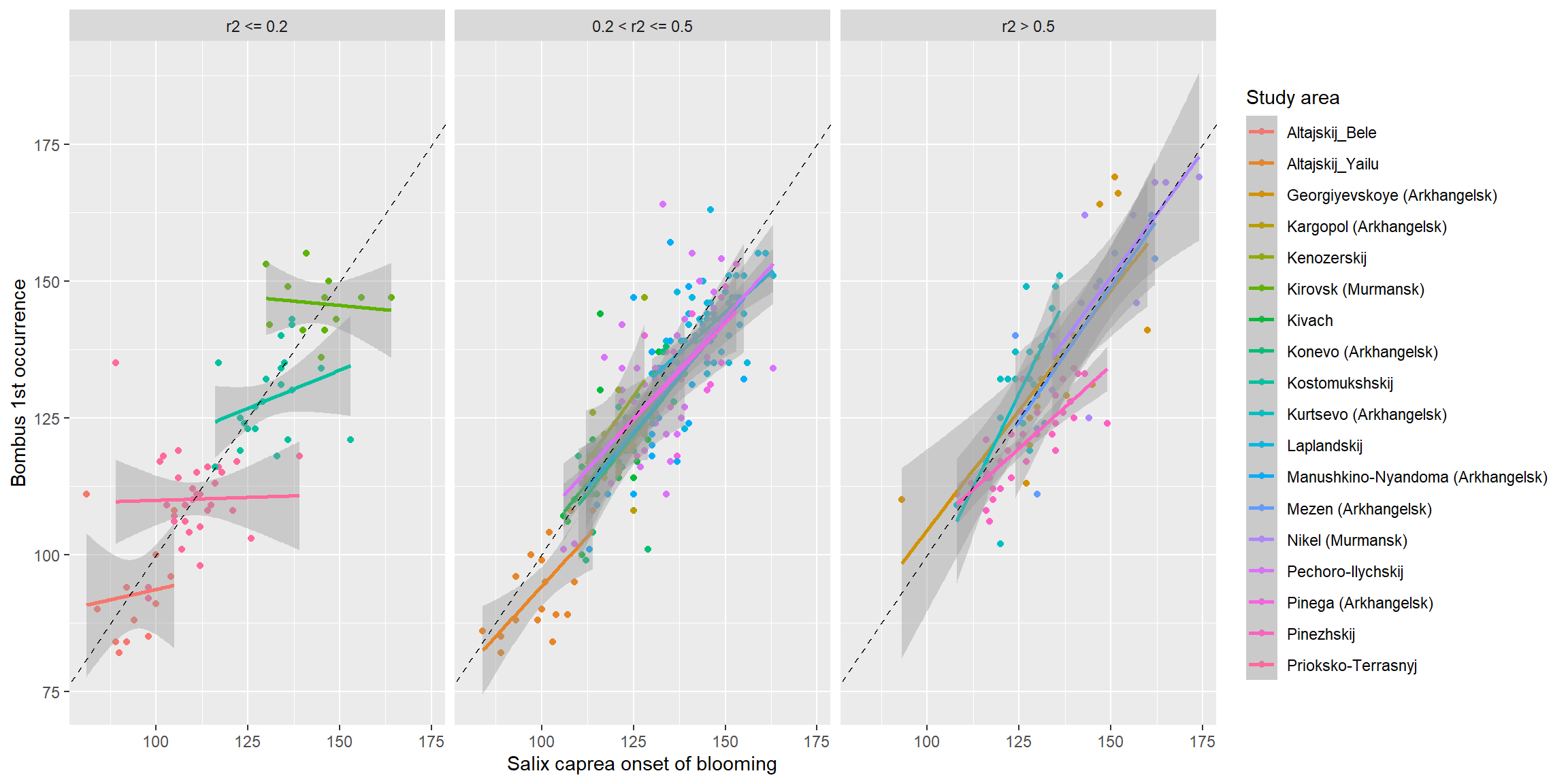
We see that for those study sites that have a strong relationship
between the first occurrence of bumblebees and the onset of blooming in
willows (i.e. those models where r2 > 0.5), these two
phenological events are tightly linked and highly synchronous! Indeed,
it seems that in many study sites, goat willows may provide the food for
the first appearing bumblebees in early spring!