Overview

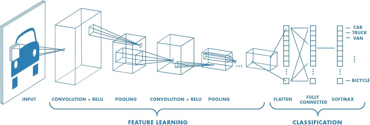
Today’s goal: to understand the steps of a Convolutional Neural Network (CNN)

Resources

Wikipedia about kernel image_processing

1 Introduction

In this practical you will “manually” follow the steps of a Convolutional Neural Network (CNN) yourself. Note that in this practical we will not actually train a CNN, but just go through the various underlying layer types to get a feeling about what happens “under the hood” of a CNN.

We will take two small top-down images of a grass pasture and a forest as an example for this practical. We will showcase with some simple filters and pooling that we can distinguish the two images and finally come to a grass- and forest-probability for both images. This practical is aimed at familiarizing yourself with the working of a CNN, but it is not aimed at improving your coding skills per se. That is why many R scripts are provided to you.

2 Setting up

Exercise 15.2a

Start by downloading the grass.jpg and forest.jpg files from Brightspace > Image analyses > Data > Images 2, save them in a new directory that you intend to use for this practical (e.g. data / raw / images2.

To load in the images, mutate and plot them we need the tidyverse, imager, gridExtra and scales packages. Install the packages if needed and then load them.

Load the grass and forest image into R as two separate cimg objects.

# Load libraries
library(tidyverse)
library(imager)
library(gridExtra)
library(scales)

# load images
grass <- load.image("data/raw/images2/grass.jpg")
forest <- load.image("data/raw/images2/forest.jpg")

3 Exploration

Exercise 15.3a

Inspect the structure of your newly loaded objects using the str function.

str(grass)

##  'cimg' num [1:50, 1:50, 1, 1:3] 0.1961 0.3843 0.4902 0.451 0.0549 ...

str(forest)

##  'cimg' num [1:50, 1:50, 1, 1:3] 0.478 0.58 0.624 0.671 0.584 ...

We can also plot the images to see what they look like in R. You can do this either in base R or with ggplot. When you use ggplot you first need to convert the arrays to data.frames or tibbles and convert the RGB values to the corresponding hexadecimal colour code (column “colCode”).

grassdf <- as.data.frame(grass, wide="c") %>%
  as_tibble() %>%
  mutate(colCode = rgb(c.1, c.2, c.3))
grassdf

## # A tibble: 2,500 × 6
##        x     y    c.1   c.2    c.3 colCode
##    <int> <int>  <dbl> <dbl>  <dbl> <chr>  
##  1     1     1 0.196  0.4   0      #326600
##  2     2     1 0.384  0.6   0.0275 #629907
##  3     3     1 0.490  0.694 0.0667 #7DB111
##  4     4     1 0.451  0.6   0.133  #739922
##  5     5     1 0.0549 0.157 0      #0E2800
##  6     6     1 0.110  0.239 0.0235 #1C3D06
##  7     7     1 0.314  0.518 0.0941 #508418
##  8     8     1 0.349  0.592 0      #599700
##  9     9     1 0.337  0.545 0      #568B00
## 10    10     1 0.384  0.529 0.0235 #628706
## # ℹ 2,490 more rows

forestdf <- as.data.frame(forest, wide = "c") %>%
  as_tibble() %>%
  mutate(colCode = rgb(c.1, c.2, c.3))
forestdf

## # A tibble: 2,500 × 6
##        x     y   c.1   c.2   c.3 colCode
##    <int> <int> <dbl> <dbl> <dbl> <chr>  
##  1     1     1 0.478 0.655 0.282 #7AA748
##  2     2     1 0.580 0.765 0.388 #94C363
##  3     3     1 0.624 0.808 0.431 #9FCE6E
##  4     4     1 0.671 0.855 0.478 #ABDA7A
##  5     5     1 0.584 0.773 0.384 #95C562
##  6     6     1 0.624 0.812 0.412 #9FCF69
##  7     7     1 0.631 0.816 0.4   #A1D066
##  8     8     1 0.631 0.820 0.392 #A1D164
##  9     9     1 0.627 0.816 0.384 #A0D062
## 10    10     1 0.545 0.733 0.294 #8BBB4B
## # ℹ 2,490 more rows

Here, we first convert the objects grass and forest into a data.frame, which includes the ‘x’ and ‘y’ value of the position of each pixel, and where the values of the 3 layers (R, G and B) will be stored in columns that will be named ‘c.1’, ‘c.2’ and ‘c.3’ (see the prefix “c” passed on to the argument wide). Then, the values of columns ‘c.1’, ‘c.2’ and ‘c.3’ are used to get a hexidecimal colour code using the function rgb. We can now plot the images:

p1 <- ggplot(data = grassdf,
             mapping = aes(x = x, y = y)) +
  geom_raster(aes(fill = colCode)) +
  scale_fill_identity() +
  ggtitle("Grass")
p2 <- ggplot(data = forestdf,
             mapping = aes(x = x, y = y)) +
  geom_raster(aes(fill = colCode)) +
  scale_fill_identity() +
  ggtitle("Forest")
grid.arrange(p1, p2, nrow = 1)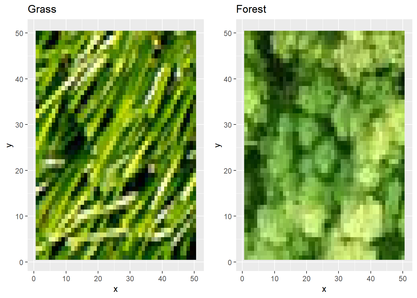

If you compare these plots to the actual images (e.g., when you open them with Windows viewer) you’ll notice that these are plotted upside-down.

Why are the images plotted upside-down?

This tells us that the coordinate indexing of images always starts in the top left corner (instead of the bottom left as ggplot assumes).

We can fix the upside-down-plotting by reversing the y axis of the plots.

p1 <- p1 +
  scale_y_continuous(trans = scales::reverse_trans())
p2 <- p2 +
  scale_y_continuous(trans = scales::reverse_trans())
grid.arrange(p1, p2, nrow = 1)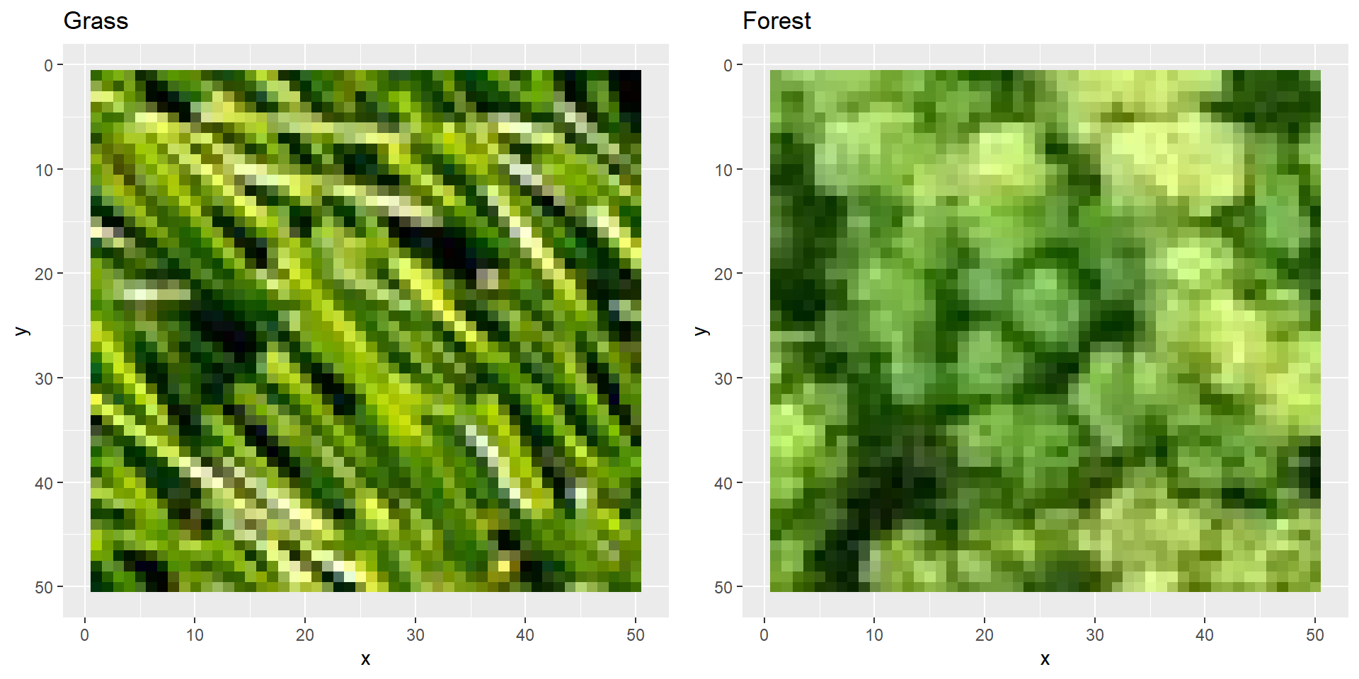

That’s more like it!

4 Pre-process

In real-life CNNs all the three colour channels (R,G,B) are often used as input data. However, for the sake of simplicity and because our two images are probably easily distinguishable, let’s convert these three colour channels to one dimension: grayscale.

grass  <- grayscale(grass)
forest <- grayscale(forest)

Let’s plot these images again.

Which function in our previous code do we now need to change?

We now need to use the grey function instead of the rgb function to convert the colour values to hexadecimal colour codes.

If we’re going to plot transformed versions of these images more often it will require a lot of repetitive code every time. So… let’s first make a function for it and then apply it to the converted images: we call this name this function plotBoth. We will make sure to scale the grey values before converting it to hexadecimal code, because later on during the transformation layers these values can become larger than 1. We do this by dividing the values by the maximum value across the images. We define the function such that it plots 2 greyscale images next to each other (grass and forest):

plotBoth <- function(grass, forest) {
  # Get max values across both images
  maxv <- max(grass, forest)
  
  # Convert to tibble
  grassdf <- grass %>%
    as.data.frame() %>%
    as_tibble() %>%
    mutate(colCode = value / maxv, # now max is 1
           colCode = grey(colCode))
  forestdf = forest %>%
    as.data.frame() %>%
    as_tibble() %>%
    mutate(colCode = value / maxv,
           colCode = grey(colCode))  
  
  # Create plots
  p1 <- ggplot(data = grassdf,
               mapping = aes(x = x, y = y)) +
    geom_raster(aes(fill = colCode)) +
    scale_fill_identity() +
    ggtitle("Grass") +
    scale_y_continuous(trans = scales::reverse_trans())
  p2 <- ggplot(data = forestdf,
               mapping = aes(x = x, y = y)) +
    geom_raster(aes(fill = colCode)) +
    scale_fill_identity() +
    ggtitle("Forest") +
    scale_y_continuous(trans = scales::reverse_trans())
  
  # Plot both images
  grid.arrange(p1, p2, nrow = 1)
}

Let’s test the function by plotting both images next to each other using the function defined above:

plotBoth(grass, forest)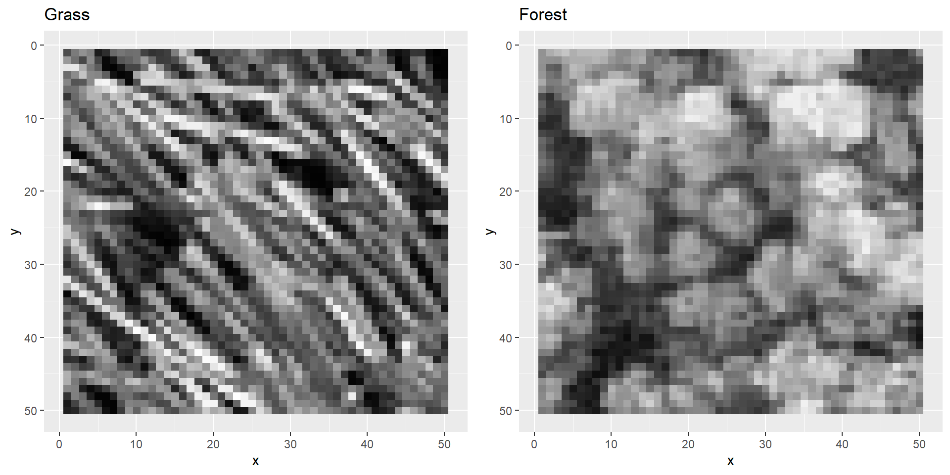

Now we are ready to put our input layers into the CNN. Remember that in this practical we imagine that we have already trained a very simple CNN and that we are going through the steps of how this CNN computes the class probabilities for each image you feed into it.

5 Layers

5.1 Convolution

The first layer of a CNN is often a Convolution Layer. The naming is actually a bit misleading, because mathematically this layer is not performing convolution. What this layer technically does is performing a sliding sum of element-wise matrix multiplications with multiple convolution filters, so more like a dot product. For one simple convolution filter (in yellow) and a very small image (green) this process is visualized in this animation:

Why is the convolved feature smaller than the input image?

The convolved value of each sliding window step will be assigned to the center element of the convolution filter. This means that you’ll lose rows and columns at the edges of your image. If you use a larger convolution filter then you’ll lose more rows and columns than in this example. If the sliding filter moves with strides greater than 1 than the resulting convolved feature will be even smaller.

The filters that are used during convolution are trained during the epochs of training your CNN. If you put multiple layers of convolution after each other the CNN is able to extract more and more complicated features from the image. However, our images are actually quite easily distinguishable with only one filter.

What is the striking difference between our two images?

The grass has more edges than the trees. An edge-detection filter will therefore most likely work well as a first step to distinguish both images. Of course, other filters might also perform well or even better.

Now that we got a feeling for which filter type will be useful for distinguishing grass from forest, let’s create three of them. Again, note that these filters are in practice trained values and you don’t have to come up with them yourself. For some common first-order convolutional filters see this Wikipedia page.

flt1 <- matrix(c(1, 0,-1,
                 0, 0, 0,
                -1, 0, 1),
               ncol = 3)
flt1

##      [,1] [,2] [,3]
## [1,]    1    0   -1
## [2,]    0    0    0
## [3,]   -1    0    1

flt2 <- matrix(c(0, 1, 0,
                 1,-4, 1,
                 0, 1, 0),
               ncol = 3)
flt2

##      [,1] [,2] [,3]
## [1,]    0    1    0
## [2,]    1   -4    1
## [3,]    0    1    0

flt3 <- matrix(c(-1,-1,-1,
                 -1, 8,-1,
                 -1,-1,-1),
               ncol = 3)
flt3

##      [,1] [,2] [,3]
## [1,]   -1   -1   -1
## [2,]   -1    8   -1
## [3,]   -1   -1   -1

flt1 <- as.cimg(flt1)
flt2 <- as.cimg(flt2)
flt3 <- as.cimg(flt3)

Okay, let’s actually perform the convolution. Take again a good look at the convolution animation to understand what is computed during this operation. To compute to convolution of an image with a certain filter you can use the convolve function of the imager package. Note that this function automatically applies some padding around the image to make sure that the convolved image has the same number of pixels as the original (in this case 50x50px). The “basic” convolution operation does not do that and would return a 48x48px image, because our filters are 3x3px we lose 2 rows and 2 columns at the edges. In a CNN you can choose to apply padding or not.

Exercise 15.5a

Perform the convolution for both grass and forest, and do this for every filter. Name your resulting convolved objects grass1, grass2, grass3, forest1, forest2, forest3.

# Apply filters on grass image
grass1 <- imager::convolve(im = grass, filter = flt1)
grass2 <- imager::convolve(im = grass, filter = flt2)
grass3 <- imager::convolve(im = grass, filter = flt3)

# Apply filters on forest image
forest1 <- imager::convolve(im = forest, filter = flt1)
forest2 <- imager::convolve(im = forest, filter = flt2)
forest3 <- imager::convolve(im = forest, filter = flt3)

5.2 ReLU

Maybe you’ve tried to plot the convolved images after the next step and encountered an error. Well done! Because this is partly why we first need to perform a next step. The convolution layers are often followed by an activation function before giving the output of the nodes to the next layers. A common activation function that is often used is the ReLU function (rectified linear unit). What this layer basically does is setting all negative values of your convolved images to zero.

Suppose that you have a vector x with values -10, -9, …, 9, 10, then you can apply the ReLu filter yourself on a copy of x (y) by setting all negative values to a value 0:

x <- -10:10
y <- x
y[y < 0] <- 0
plot(x, y, type = "b")

Why do you think it is good practice to use a ReLU layer after convolution?

This makes the computation and fitting of your CNN much more efficient.

Exercise 15.5b

Apply the ReLU function yourself on all the convolved grass and forest objects. When you’re done, plot the convolved images using your plotBoth function to take a look at them.

grass1[grass1 < 0] <- 0
forest1[forest1 < 0] <- 0
plotBoth(grass1, forest1)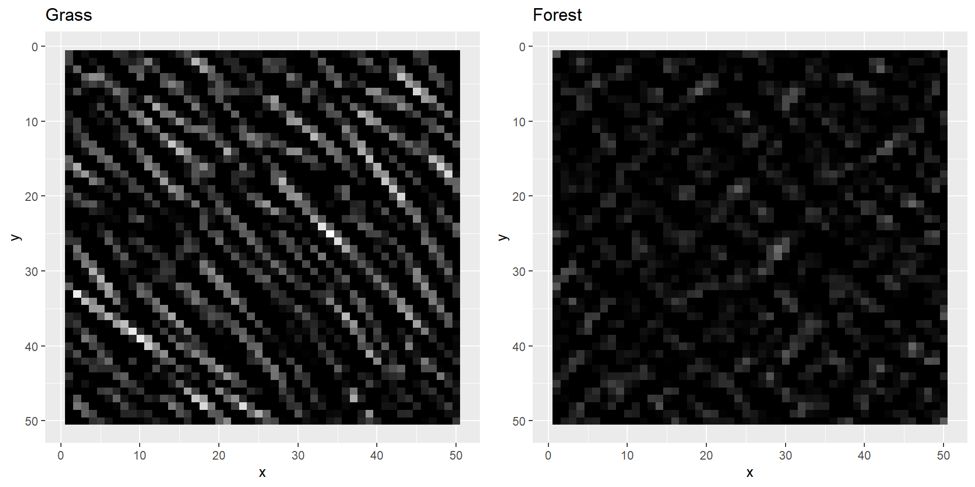

grass2[grass2 < 0] <- 0
forest2[forest2 < 0] <- 0
plotBoth(grass2, forest2)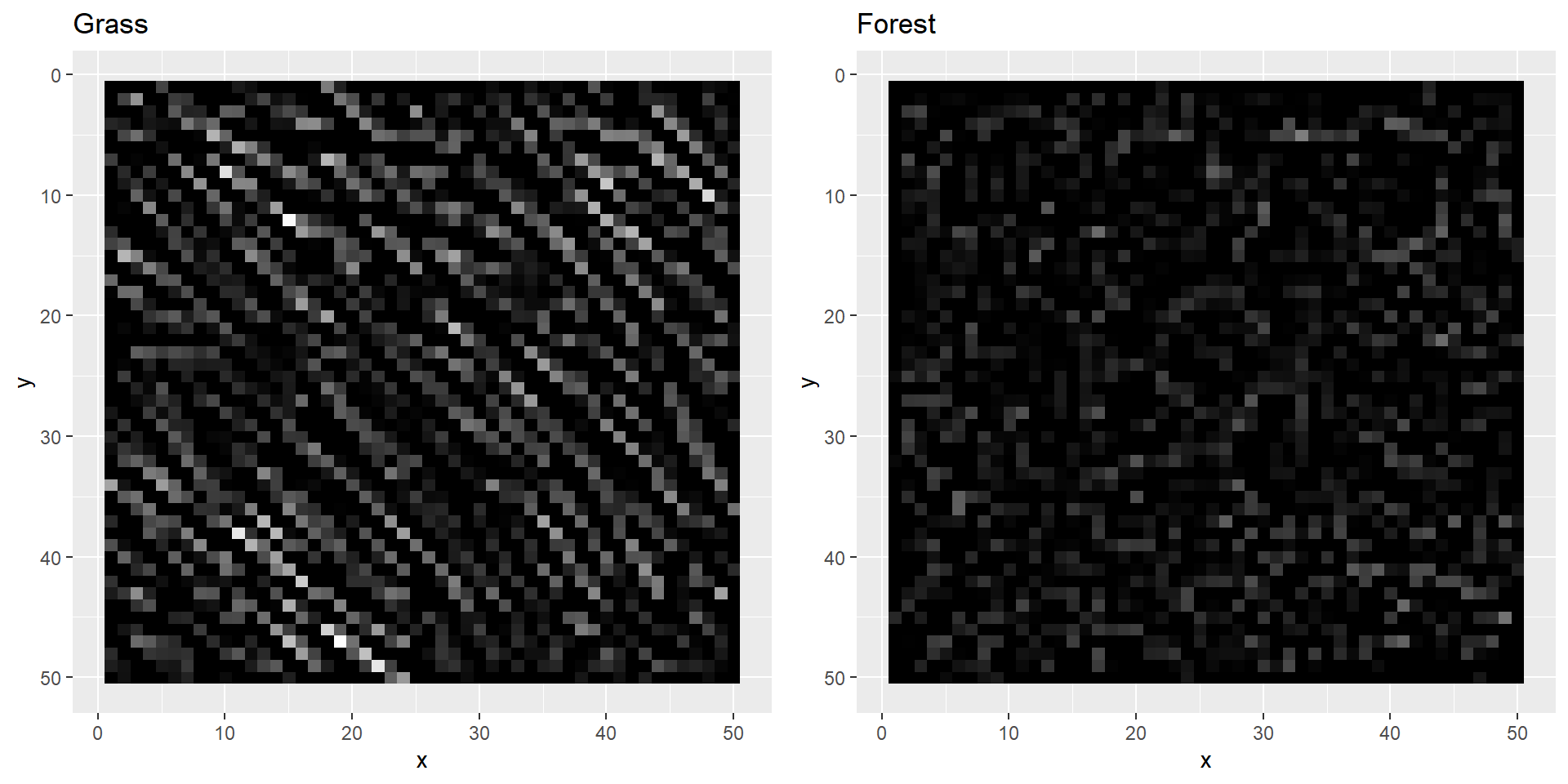

grass3[grass3 < 0] <- 0
forest3[forest3 < 0] <- 0
plotBoth(grass3, forest3)

As you can probably see, our filters highlighted the edges of our two images. Just as we hoped, the grass image lights up much more than the forest image. We can now try to use the computed values to try and distinguish both images. However, for that we need some more layers.

5.3 Max pooling

Another very common layer is a pooling layer, often placed after a convolution layer. This layer is quite similar as a convolution layer, again using a sliding window approach. The idea behind a pooling layer is to reduce the size of the convolved images through down-sampling. In contrast to the convolution layer, the pooling layer often uses a larger window that moves through the image with larger and non-overlapping strides (to make sure the pooled image is substantially smaller than its input). Most of the time the maximum value per window is returned, hence the name: max pooling.

Why do you think it is good practice to use a pooling layer in your CNN?

To reduce the noise and extract the most important patterns from the image, which also makes sure it is easier to compare various images with each other that differ in orientation. Furthermore, this again makes the computation and fitting of your CNN much more efficient.

We can create a function that applies the max pooling:

maxPool <- function(im, size, stride) {
  pool <- as.cimg(matrix(rep(NA_real_, (dim(im)[1]/stride * dim(im)[2]/stride)),
                         ncol = dim(im)[2]/stride))
  
  for(i in seq_along(pool[1,])) {
    for(j in seq_along(pool[,1])) {
      pool[i,j,1,1] <- max(im[((i-1)*stride+1):(i*size),
                              ((j-1)*stride+1):(j*size),
                              1,
                              1])
    }
  }
  
  return(pool)
}

Why is it not useful to apply another ReLU layer after this pooling layer?

There are already no zeroes left in our data, so applying a max pooling will not result in any zeroes as well.

Exercise 15.5c

See if you can understand what is happening in the function defined above. Apply this max pooling layer on all your convolved objects by using a window of 5x5px with strides of 5. Plot the pooled images afterwards to check if the output makes sense. Name your pooled cimg objects grassPool1, forestPool1 etc.

grassPool1 <- maxPool(grass1, size = 5, stride = 5)
grassPool2 <- maxPool(grass2, size = 5, stride = 5)
grassPool3 <- maxPool(grass3, size = 5, stride = 5)

forestPool1 <- maxPool(forest1, size = 5, stride = 5)
forestPool2 <- maxPool(forest2, size = 5, stride = 5)
forestPool3 <- maxPool(forest3, size = 5, stride = 5)

plotBoth(grassPool1,forestPool1)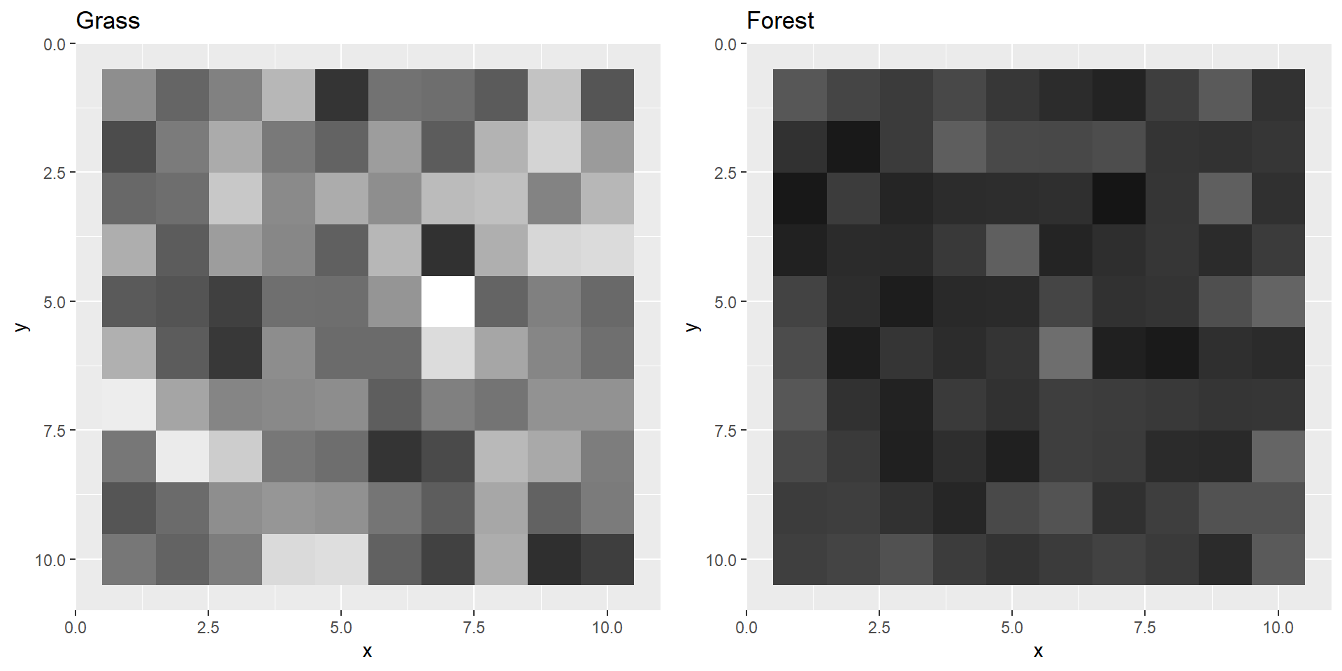

plotBoth(grassPool2,forestPool2)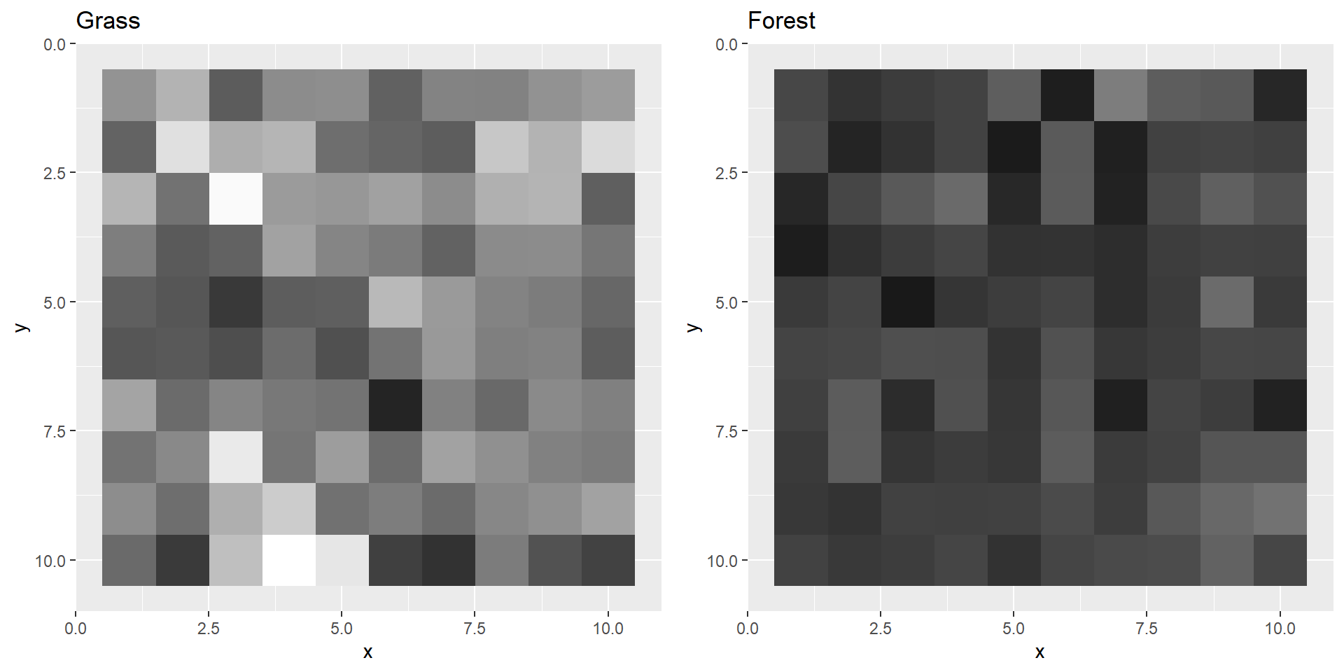

plotBoth(grassPool3,forestPool3)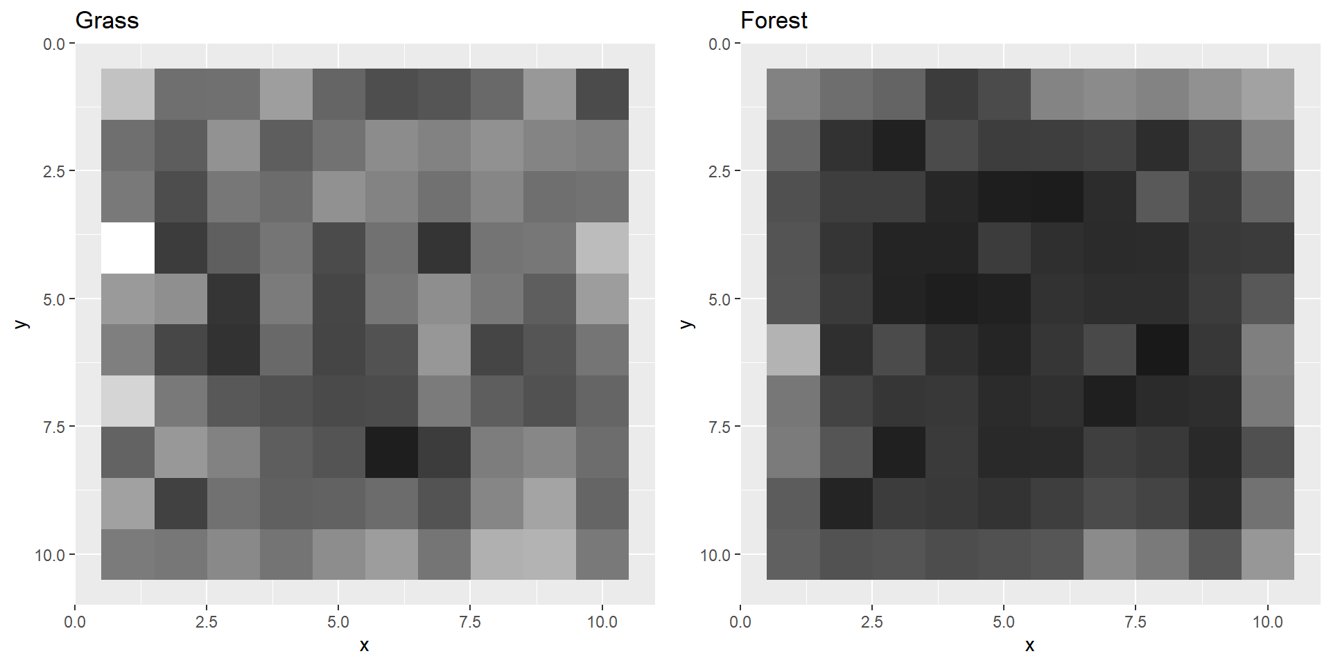

In actual CNNs there are usually multiple convolution, activation and pooling layers after each other. The more layers, the “deeper” your neural network becomes. Deep neural nets are able to detect more difficult patterns. CNNs with 50 layers are for example very common. For our example these few layers will probably suffice.

5.4 Flattening

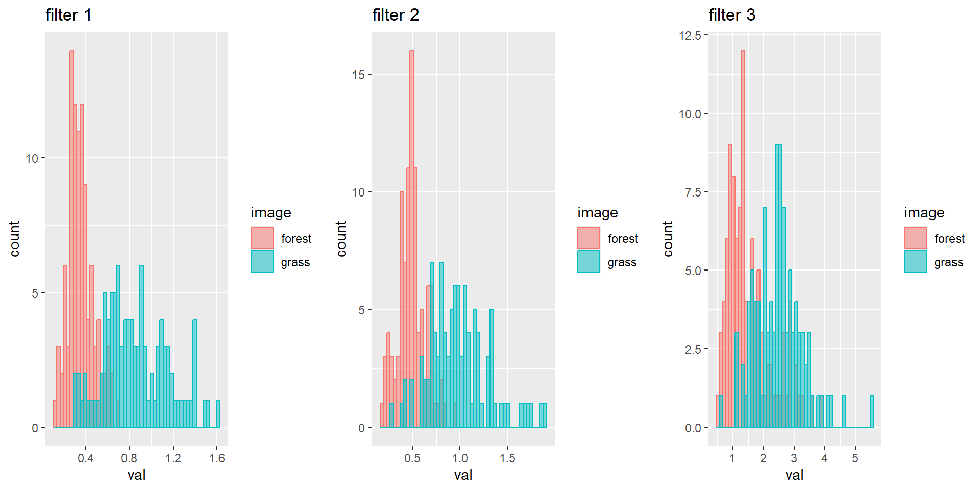
After the last pooling layer we have finished the feature learning part of the CNN and now arrive at the final part: the actual classification. In order to perform the classification we need to treat the pooled images as feature vectors, therefore we need to “flatten” our 2D images into 1D vectors. This can be performed easily in R with the as.vector function, name them grassFlat1, forestFlat1 etc. After you’ve flattened all the 6 pooled matrices, create 3 histograms of the grass and forest image combined per filter:

# Convert to vectors
grassFlat1  <- as.vector(grassPool1)
forestFlat1 <- as.vector(forestPool1)
grassFlat2  <- as.vector(grassPool2)
forestFlat2 <- as.vector(forestPool2)
grassFlat3  <- as.vector(grassPool3)
forestFlat3 <- as.vector(forestPool3)

# Merge to tibbles
Flat1 <- tibble(val = list(grassFlat1, forestFlat1), 
              image = c("grass","forest")) %>% 
  unnest(val)
Flat2 <- tibble(val = list(grassFlat2, forestFlat2), 
              image = c("grass","forest")) %>% 
  unnest(val)
Flat3 <- tibble(val = list(grassFlat3, forestFlat3), 
              image = c("grass","forest")) %>% 
  unnest(val)

# Plot
p1 <- ggplot(Flat1, aes(x=val, color=image, fill=image)) +
  geom_histogram(position="identity", alpha=0.5, bins=50) +
  ggtitle("filter 1")
p2 <- ggplot(Flat2, aes(x=val, color=image, fill=image)) +
  geom_histogram(position="identity", alpha=0.5, bins=50) +
  ggtitle("filter 2")
p3 <- ggplot(Flat3, aes(x=val, color=image, fill=image)) +
  geom_histogram(position="identity", alpha=0.5, bins=50) +
  ggtitle("filter 3")

grid.arrange(p1, p2, p3, nrow = 1)

What do we learn from these histograms?

The grass image has on average much higher values than the forest image for every filter.

5.5 Fully connected

After the flattening layer, all nodes are combined with a fully connected layer. This fully connected layer is actually a regular feed-forward neural network in itself. The output of this fully connected layer is a value for each class the CNN is trained to predict (in our case grass and forest). In reality this fully connected layer can become very complex, and have hidden fully connected layers prior to it. However, as we’ve already seen in the histograms, our images are easily distinguishable. So now let’s assume that we can compute the score for the both classes by simply using the sum of the three flattened vectors (which would be the outcome of the fully connected layer when every node in the previous layer gets a weight of 1 and the bias term is 0). The grassRef and forestRef values are what we assume that the CNN learned in the training phase.

# Get sum across layers
grassValue  <- sum(c(grassFlat1, grassFlat2, grassFlat3))
forestValue <- sum(c(forestFlat1, forestFlat2, forestFlat3))

# Set reference values
grassRef  <- 360
forestRef <- 180

# Compute absolute difference from references
grass_grassScore  <- 1 - abs(grassRef-grassValue)
grass_forestScore <- 1 - abs(forestRef-grassValue)

forest_grassScore  <- 1 - abs(grassRef-forestValue)
forest_forestScore <- 1 - abs(forestRef-forestValue)

Why does our fully connected layer output 4 score values?

For every image the CNN computes the probability for both the grass and the forest class. With two images this results in four values.

5.6 Activation

Finally, after classification in the fully connected layer, the class probabilities can now be computed for every image. For this we use again an activation function, just like the ReLU function. However, at the end of the CNN a Softmax activation layer is often used. This activation function has the nice property that you can consider the output values as probabilities (values between 0-1) and it scales well with many classes, so that the class with the largest value gets a proportionally much higher value than the other classes. The Softmax function is: \(\frac{e^{x_i}}{\sum^n_{j=1} e^{x_j}}\), where \(x_i\) is the value of class \(i\) of the total of \(n\) classes that the CNN is trained for. Now compute the grass and forest probability yourself for both images.

# Softmax function
grass_grassProb <-  exp(grass_grassScore) / sum(exp(grass_grassScore), exp(grass_forestScore))
grass_forestProb <- exp(grass_forestScore) / sum(exp(grass_grassScore), exp(grass_forestScore))

forest_grassProb <-  exp(forest_grassScore) / sum(exp(forest_grassScore), exp(forest_forestScore))
forest_forestProb <- exp(forest_forestScore) / sum(exp(forest_grassScore), exp(forest_forestScore))

# Show values
matrix(c(grass_grassProb, grass_forestProb, 
         forest_grassProb, forest_forestProb),
       ncol = 2,
       dimnames = list(image = c("grass","forest"),        # Row label and names
                       probability = c("grass","forest"))) # Col label and names

##         probability
## image           grass       forest
##   grass  1.000000e+00 2.320913e-25
##   forest 6.714184e-79 1.000000e+00

How does the behaviour of the Softmax function differ compared to e.g. logistic regression?

The probabilities per class depend on the values of the other classes. This means that two CNNs that are trained to detect forest with the same input data, but differ in the other classes that they are trained to detect, will most likely return different probabilities for the forest class on the same image.

6 Recap

During this practical you have taken a look under the hood of a CNN to see what happens when it predicts the class probabilities of images. Hopefully you have now a better feeling about how a CNN works and about its philosophy. Furthermore, you’ll probably also be pleased to know that from now on all the convolution, pooling, flattening, connecting and activation layers will be computed for you with some very simple functions in only a few lines of code. Something to look forward to…

An R script of today’s exercises can be downloaded here

Understanding convolutional neural networks