The free and open-source software
R is widely
used in many fields of science and beyond. It is an extremely versatile
programming language, as well as an interactive
environment for data exploration and statistical computing, especially
when combined with the functionality that
RStudio provides.
If you have not installed R and RStudio yet, you can download the
latest versions from the
R and
RStudio
websites.
In generating this document, we used R v4.5.2, and RStudio
v2026.01.1-403. For a Windows system, you can download the corresponding
versions of R and RStudio from
here
and
here,
respectively.
On most computers, the installation of both R and RStudio using all
default settings will work out just fine. Thus, if you use your own
computer on which you have appropriate admin rights, you can install R
first, and then RStudio, using the default settings. However, if you run
into problems installing (or using) R when installed in the default way;
then follow the steps as outlined
here.
R is basically a scripting language, providing a means to make and
run scripts. Scripting is essential for quality control
and transparency of data processing, and it is more and more a
requirement to ensure transparency and repeatability of data processing
in science. Our end goal should not just be to “do stuff”, but to do it
in a way that anyone can easily and exactly replicate our workflow and
results. The best way to achieve this is to write scripts.
R is a dynamic or interpreted
programming language, which means that - contrary to compiled languages
like C++ - you don’t need a compiler to first create a
program from your code before you can use it. R interprets your code
directly, so that you simply can write code and run it. This makes the
development cycle fast and easy.
RStudio is more than simply a graphical user interface (GUI) for R;
it is an open-source integrated development environment (IDE) that
includes a console, syntax-highlighting editor that supports direct code
execution, as well as tools for plotting, history, debugging, workspace
management and version control.
Always load R through the RStudio IDE!
2 Pane overview
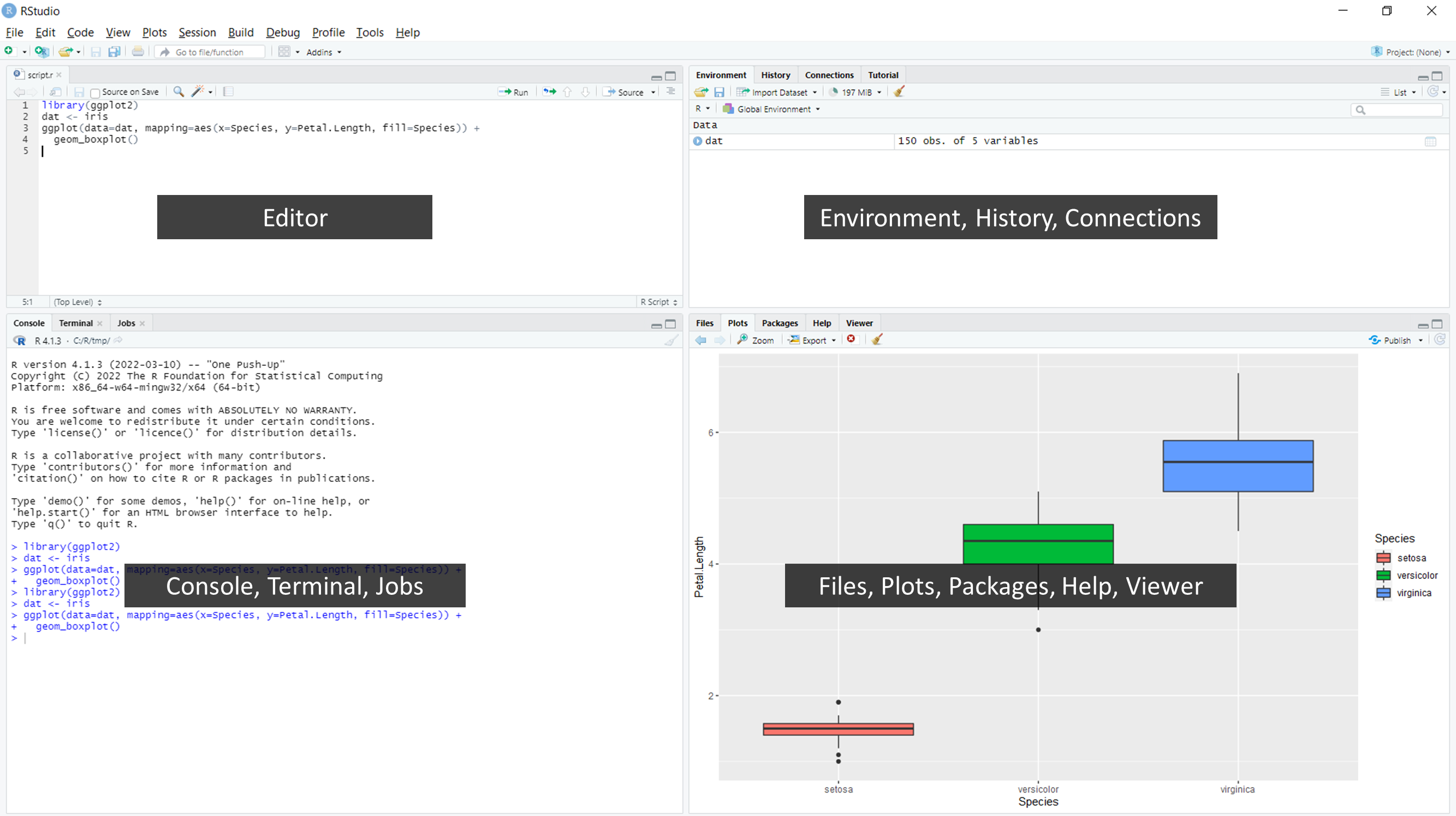
RStudio displays multiple panes (or panels, windows) in which
different types of content is displayed. In the default setting, if you
have not yet opened a script, there are 3 panes, yet there are 4 when
you have opened a script. In that case, the top-left window contains a
script editor, the console is at the
bottom-left, the environment window (showing what is
stored in memory) is at the top-right, and a plotting
window is bottom-right. Some panels have multiple tabs
that include other useful features such as help and
information on (available and loaded) packages
etc.:
You can change the location of panels and what tabs are shown under
View > Panes > Pane Layout. Via Tools > Global
options > Appearance, you can change to looks of the GUI, e.g.,
used colours.
The console is the heart of R. Here is where R actually evaluates
code. If the last character you see is
> (a prompt) it
indicates that R is waiting for new input (and thus has finished any
prior task). You can type code directly into the console after the
prompt and get an immediate response. For example, if you type
1+1 into the console and press enter, you’ll see that R
immediately gives an output of 2.
In the console, if instead of R’s prompt symbol
> you see the symbol
+, then it means that R expects you to
complete the current command! If you want to abort the command
(e.g. when the script is wrong, for example when you do not have
matching closing brackets), you can hit the Esc key on the
keyboard when your cursor is at the console.
The script editor lets you work with source script files. Here, you
can enter multiple lines of code, and save your script file to disk (R
scripts are just text files; save them with the .r
extension). The RStudio script editor recognizes and highlights various
elements of your code, for example using different colours for different
elements, and it also helps you find matching brackets in your
scripts.
Instead of typing directly into the console, it is thus better to
enter the commands in the script editor. This way, R commands can be
recorded for future reference. To execute some code, you can either
select the code you wish to execute and click on the
Run button on the top right of the script panel, or
press a hot-key such as “Ctrl + Enter” or “Ctrl + r” on a Windows pc
(“Command + Return” on an Apple pc; below we will assume you work on a
Windows machine). To see all shortcuts in RStudio, check “Alt + Shift +
k” (or Tools > Keyboard Shortcut help). To facilitate
reproducibility of your project, write most of your code in script, and
only type directly into the console to de-bug or do quick analyses
(i.e., small tasks that do not need to be saved for future
reference).
Most of the time working in a project you will be working on scripts
in the scripts editor panel, and check output in the console or plot
panel. It is always good practice to make ample use of the
help tab, which provides the help menu for R functions.
To quickly access the help file associated to some function, use the
help() function and ? help operator. For
example, if you want to retrieve the documentation of the function
lm, you could enter the command help(lm) or
help("lm"), or ?lm or ?"lm"
(i.e., the quotes are optional).
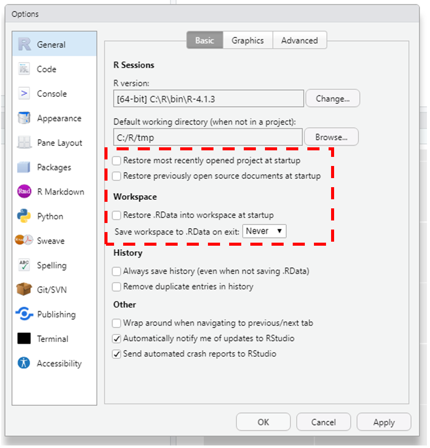
3 Configuring RStudio
It is advised to configure the settings of RStudio before you start
working on a project. By default, RStudio re-uses / restores projects,
saves history, and asks on exit whether or not to save the workspace to
file. Via Tools > Global Options > General you can
configure RStudio (see
here
for explanation of the options). If you keep things around in your
workspace, things will get messy, and unexpected things will happen. It
is therefore good practice to uncheck all
restore checkboxes and set the Save workspace to .RData on
exit to Never, so that when you start RStudio you
start with a clean sheet:
This forces you to work in a clean and structured way, thereby
increasing the transparency and reproducibility of your project! This is
not only benefiting reproducible science, it also will help your future
self: when you resume a project after some break, you can easily pick up
right where you left off when you work in a transparent and reproducible
way.
4 Packages
Packages are collections of functions and data sets developed by the
community: they increase the power of R by improving existing base R
functionalities, or by adding new ones. There are thousands contributed
packages available, each with its own suite of functions and built-in
datasets. A package first needs to be installed on your pc, and
then loaded into the R session, before you can use the
functions that the package offers. Packages can be installed on your pc
using the install.packages() function, via the Packages
tab in the bottom-right panel of RStudio, or via Tools >
Install Packages. Once you have installed a package on your pc you
never need to install it again (unless you want to install a new version
of the package). To load a package into the R session, you use the
library() function.
Sometimes, different packages contain functions with the same name.
In that case, the order in which you load the packages influences which
function is being executed once called. Usually, you see warnings
printed to the console when this is the case.
You can call a function from a specific package using
packagename::functionname(), for example, the function
select is defined in the dplyr package as well
as the raster package: in order to explicitly use the
select function from the dplyr package you can
run: dplyr::select().
The fundamental idea behind a robust, reproducible analysis is a
clean, repeatable script-based workflow (i.e. the sequence of tasks from
the start to the end of a project) that links raw data through to clean
data and to final analysis outputs. Most analyses will be re-run many
times before they are finished (and perhaps a number of times more
throughout the review process), so the smoother and more automated the
workflow, the easier, faster and more robust the process of repeating it
will be.
A project often consists of a multitude of files; from input data,
documentation and scripts to output files, tables, figures and reports.
It is thus best to think about a good file system organisation, and
informative, consistent naming of materials associated with your
analysis, before you start any project. The BES guide lists a few
principles of a good analysis workflow:
Start your analysis from copies of your raw data;
Any cleaning, merging, transforming, etc. of data should be done in
scripts, not manually;
Split your workflow (scripts) into logical thematic units. For
example, you might separate your code into scripts that (i) load, merge
and clean data, (ii) analyse data, and (iii) produce outputs like
figures and tables;
Eliminate code duplication by packaging up useful code into custom
functions. Make sure to comment your functions thoroughly, explaining
their expected inputs and outputs, and what they are doing and why;
Document your code and data as comments in your scripts or by
producing separate documentation;
Any intermediary outputs generated by your workflow should be kept
separate from raw data.
It is best to keep all files associated with a particular project in
a single root directory: thus one folder for one project! RStudio’s
R projects offer a great way to keep
everything together in a self-contained and portable (i.e., so they can
be moved from computer to computer) manner, allowing internal pathways
to data and other scripts to remain valid even when shared or moved.
There is no single best way to organise a file system. The key is to
make sure that the structure of directories and location of files are
consistent, informative and works for you. The BES gives a good example
of a basic project directory structure:
The data folder contains all input data (and
metadata) used in the analysis.
The doc folder contains the manuscript.
The figs directory contains figures generated by
the analysis.
The output folder contains any type of intermediate
or output files (e.g., simulation outputs, models, processed datasets,
etc.). You might separate this and also have a cleaned-data folder.
The scripts directory contains R scripts with
function definitions.
The reports folder contains files (e.g. RMarkdown)
that document the analysis or report on results.
The scripts that actually do things are stored in the root
directory, but if your project has many scripts, you might want to
organise them in a directory of their own.
Never ever touch (edit) raw data! Store raw data separately
and permanently in a (sub-)folder, e.g. in
data/raw/. Process (e.g., clean, filter,
select, change) the raw data using scripts, and optionally save
processed data in a separate sub-folder, e.g. in
data/processed/.
On your computer, create a folder with directory structure (you may
include the full folder structure as shown above, but minimally the
data, output and scripts folders) where you
will keep your files for the tutorials the coming weeks.
If RStudio and R are not installed on your pc yet, install it using
the information given above. Make sure that RStudio is configured such
that when you start RStudio, you start with a clean sheet (and thus do
not restore your workspace at start-up; see above).
In RStudio, go to File > New Project and choose
Existing Directory. Browse to the root of the new file
directory structure that you just created and click Create
Project. A new R session starts, and in the Files
tab in the bottom-right panel, you’ll see that your files location is
now actually in the just created project folder.
Create a new R script using File > New File > R
Script, or by clicking the New File icon directly below the File
menu option, and R Script. Save it in the folder “scripts/” as file
“day_01.r”. Code the exercises below in this script. During the coming
days in this course, start each day by making a new script file with a
clear name, saved in the “scripts/” folder, code that day’s exercises in
that script.
When you have created your project, you only have to double-click (or
via File > Open Project) on the generated
.Rprj file to open the project in RStudio and continue
working. When you click on the .Rproj file in the bottom-right
Files panel, a pop-up will appear with the settings specific to
the project. By default, RStudio’s global settings are inherited, but
you could choose to change them for the specific project (or leave them
at their defaults).
7 Working directory
An advantage of defining and using a R Project is that RStudio will
automatically set the root folder of your project directory structure as
the working directory. Thus, when you load (or save)
files from (to) disk, you can quickly and conveniently use paths
relative to this root folder, for example:
Where
Example
in the working directory
“observations.csv”
in a sub-folder
“data/raw/observations.csv”
Note the convention of using forward slashes, unlike the
Windows-specific convention of using backward slashes. This is to make
references to files platform-independent.
You can get, and set, the working directory using the functions
getwd() and setwd(), respectively.
Set the working directory for a project maximally
once, and set it to the root directory of your project.
Regularly changing the working directory (e.g., to load files) is bad
practice.
If you have to set the working directory using the
setwd() function, think carefully whether you do it in a
script or directly in the console. Consider that other people with whom
you might be collaborating do not have the same directory tree (path) as
you, and nor will you in the future when you work on a different
computer.
When manually setting the working directory, therefore do so by using
the Session > Set Working Directory pull-down option, by
typing the appropriate setwd() command in the console, or
by running setwd() from a script.
Exercise 1.7a
Set the working directory to your project root folder using any of
the above-mentioned methods, and check that the working directory is set
to the correct folder using getwd().
8 Data frames
Before we enter the tidyverse universe, let’s first
have a look at one of the most important, and basic, data
structures in base R: data frames. Let’s create a
data.frame called df and assign it 100 records with 4
properties each: id, x, y and
lab:
df <- data.frame(id = 1:100,
                 x = runif(100),
                 y = runif(100),
                 lab = rep(c("a","b","c",
                             "d","e"), 20))
Here, the column id simply holds the record number,
x and y contain random (uniform) values
(between 0 and 1), and lab contains the letters
“a”,“b”,“c”,“d”,“e” (each repeated 20 times).
Exercise 1.8a
Create the object df as specified above, and print the
data.frame to the console using:
df
while printing a data.frame, you will see
all records (here thus 100, although when the dataset
is really large R will stop showing output after a preset maximum is
reached), up to a point where the console is fully flushed with
information and the maximum is reached (usually this may take a long
time, sometimes forcing you to abort your R session and start over
again). This is what your console will look like when printing the
data.frame: not all 100 records are shown, just to top and bottom 10
(but note that on your computer the numerical values of “x” and “y” will
differ, as we generate random values here!):
##    id          x         y lab
## 1   1 0.89508851 0.9319207   a
## 2   2 0.42916998 0.9400032   b
## 3   3 0.96363656 0.3058434   c
## 4   4 0.51168831 0.8535155   d
## 5   5 0.67817580 0.6263964   e
## 6   6 0.98450613 0.2966926   a
## 7   7 0.76199356 0.7206086   b
## 8   8 0.23947016 0.8472440   c
## 9   9 0.03899944 0.2483362   d
## 10 10 0.18057906 0.2800645   e
. . .
##      id          x         y lab
## 91   91 0.50805941 0.1549644   a
## 92   92 0.17276773 0.9344424   b
## 93   93 0.75111636 0.2354497   c
## 94   94 0.90906616 0.1381533   d
## 95   95 0.04989612 0.5750344   e
## 96   96 0.30724767 0.1074442   a
## 97   97 0.82408871 0.4136451   b
## 98   98 0.12049582 0.8526272   c
## 99   99 0.05868078 0.6173500   d
## 100 100 0.89344206 0.7023502   e
You cannot directly see from the printed output what
type of data is stored in each column of the data.frame. For example,
you see that the column lab contains the values
a, b, … ,e, but are these of
class character or factor? This is not visible
without the help of a function like str, which gives an
overview of the contents of a data structure (e.g. data.frame). Check
for yourself:
str(df)
## 'data.frame':    100 obs. of  4 variables:
##  $ id : int  1 2 3 4 5 6 7 8 9 10 ...
##  $ x  : num  0.895 0.429 0.964 0.512 0.678 ...
##  $ y  : num  0.932 0.94 0.306 0.854 0.626 ...
##  $ lab: chr  "a" "b" "c" "d" ...
Here, we can see that lab contains data of type
character (for R version 4; for older versions you see that
it is of class factor). Check the ?data.frame
help file: notice that there is a stringsAsFactors function
argument that is set to the value of the system default (defaults to
TRUE prior to R version 4). This means that when a
data.frame is created, a column with values of class
character is automatically converted to class
factor, with often unwanted consequences.
Although data.frames are an important and central way of storing data
in R, the example above shows but a few examples of behaviour that are
not ideal!
9 Tidyverse
As discussed in the lectures, data scientists spend close to 80% (if
not more) of their time cleaning, massaging and preparing data: it is
simply the most time-consuming aspect in data science. Unfortunately, it
is also among the least interesting things data scientists do (i.e., it
doesn’t directly produce nice visualisations, model output, or
predictions). However, it is an inevitable part of the data science
process: we simply cannot build powerful and accurate models without
ensuring our data is well prepared!
But: lets enter the world of tidyverse! It is the most
powerful collection of R packages for preparing, wrangling, visualizing
and modelling data.
The tidyverse (see
tidyverse.org)
is an opinionated collection of R packages designed for data science.
All packages share an underlying design philosophy, grammar, and data
structures (see
here
for the manifesto on tidy data: the consistent principles that
unify the packages in the tidyverse).
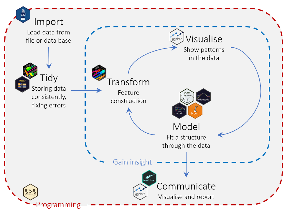
The tidyverse is actually some sort of meta-package: an umbrella for
a collection of packages that all have their own function in the
workflow of data science. For an overview of these packages, see
tidyverse.org/packages.
The following figure places the different packages into the data science
workflow:
All packages within the umbrella of tidyverse have their own
dedicated website: <packagename>.tidyverse.org (e.g., for
the tibble package that we will explore below, see:
tibble.tidyverse.org).
Exercise 1.9a
Curious to explore the tidyverse? Go ahead and install the tidyverse
package from within RStudio, using either the menu option Tools >
Install Packages, the Packages panel in the bottom-right
panel, or the install.packages function. After that, load
the package into your R session using the library function.
install.packages("tidyverse")
After installation, you have to load package using:
library(tidyverse)
When loading the tidyverse package, you will see some information on
the loaded packages (e.g. their version, and possible conflicts with
similarly-named functions from other packages).
10 Tibbles
Central to the tidyverse way of doing data science is a data format
that is an optimized version of a data.frame: a tibble.
A tibble can be used anywhere a data.frame is used (it technically
is a data.frame!). Similar to how we created the data.frame
df above, we can make it as a tibble, using the
tibble function:
tb <- tibble(id = 1:100,
              x = runif(100),
              y = runif(100),
              lab = rep(c("a","b","c",
                          "d","e"),20))
Exercise 1.10 a
Create the object tb now as a tibble as shown above, and
print it to the console using:
tb
The output printed to the console gives us a very concise yet
informative overview of the object tb: it states that it is
a tibble, with dimension 100 (records, thus rows) x 4 (columns); it
gives the classes of all shown columns (int, dbl, and
chr, see table below), shows only the top-10 rows, and at the
bottom indicates that 90 rows have been omitted from the view:
## # A tibble: 100 × 4
##       id     x      y lab
##    <int> <dbl>  <dbl> <chr>
##  1     1 0.217 0.407  a
##  2     2 0.204 0.733  b
##  3     3 0.732 0.563  c
##  4     4 0.619 0.595  d
##  5     5 0.583 0.322  e
##  6     6 0.789 0.874  a
##  7     7 0.464 0.417  b
##  8     8 0.227 0.0364 c
##  9     9 0.292 0.347  d
## 10    10 0.786 0.391  e
## # ℹ 90 more rows
Isn’t this a much more convenient behaviour than how data.frames
behave?!
The basic data types in R (many other types exist also), and how they
are shown in tibble:
type
tibble code
example
integer
<int>
-1, 0, 4
numeric/double
<dbl>
3, 0.1,
-235.4
boolean/logical
<lgl>
TRUE, FALSE
character
<chr>
"hello world", 'test'
factor
<fct>
datetime
<dttm>
For now, we do not go into the details of factors and datetime
objects, that’s for later.
Apart from showing us ample information in a concise way, tibbles
have other behaviours that are more pleasant from a data science
perspective: they do not change variable names or types (as data.frames
do when including a character vector: R versions older than v4 converted
characters by default to a factor). Moreover, while data.frames support
partial name matching, tibbles do not. For example, when you want to
retrieve the column with the name “lab” from the above-generated tibble
tb using tb$la, tibbles will throw a warning
back at you, while data.frames will try to guess what you meant. Give it
a try:
df$la
tb$la
As seen, a tibble will give errors when writing only part of a column
name (or omitting parts by mistake), decreasing the risk of selecting
wrong variables, hence resulting in a cleaner and more reproducible
process.
Another advantage of using tibbles instead of data.frames is that
subsetting or indexing them using square brackets [,], you
will always get a tibble back (yet in a data.frame it depends on your
subset what you get back). Compare the difference for yourself, by
retrieving the 4th column of both objects (if you are not familiar with
the [,] notation yet, do not bother too much about it right
now):
df[,4]
tb[,4]
Along with the above listed advantages, the Tibble package helps us
in easy handling big datasets containing complex objects, as we will see
next week. Such features enable us to treat the inherent data issues
early on, hence producing cleaner code and data, and thus a smoother
data science workflow.
Similar to the str function, tibbles can be explored
using the glimpse function, e.g.:
Above, the tb tibble was created using the
tibble function, which fills the data column-wise.
To fill data row-wise, you can use the tribble
function:
tribble(
  ~colA, ~colB,
  "a",   1,
  "b",   2,
  "c",   3
)
## # A tibble: 3 × 2
##   colA   colB
##   <chr> <dbl>
## 1 a         1
## 2 b         2
## 3 c         3
11 Data input/output
Base R already includes some functions to load (or save) data from
external sources, e.g. the functions load
(save) for .RData or .rda files, readRDS
(saveRDS) for.rds files, read.csv
(write.csv) for comma-separated files, and
read.table (write.table) or
read.delim for more generic function reading in delimited
files. The functions read.csv,read.table, and
read.delim load the data into a data.frame format
(including the default conversion of strings to factors - but see the
function argument stringsToFactors).
Tidyverse also contains some packages (readr and
readxl) to load data from an external file: the
advantage is that the tidyverse functions are often faster than the base
R functions, have much better error handling, and mostly that they
directly load data into a tibble! This provides an improvement
over the standard file importing methods and significantly improves
computation speed. The following table gives an overview of several
useful importing/exporting functions in base R and tidyverse (here we
omit the read.csv and write.csv functions, as
the tidyverse equivalents - which you can recognize by the use of the
underscore instead of a dot, thus read_csv instead of
read.csv - are preferred due to their advantages):
File Extension
Reading
Writing
.csv
read_csv()
write_csv()
several
read_delim()
write_delim()
.xlsx
read_xlsx()
write_xlsx()
.rds
read_rds()
write_rds()
All of the functions in the table above except for
read_xlsx() and write_xlsx() are from the
readr package. Function read_xlsx() is
from the readxl package, which is installed when you
install tidyverse, yet you have to load the package first (as it is not
loaded when running library(tidyverse)). Function
write_xlsx() is from the writexl package,
which you need to first install and then load before using it. Note that
in general it may be better to stick to plain-text delimited files such
as .csv instead of loading Excel workbooks into R!
Exercise 1.11a
Save the file Forest biomass data.csv from
Brightspace (Skills > Datasets > Forest) to the folder
“data/raw/forest/” in the project directory you created on your
pc. This file contains data of aboveground biomass in Eurasian forests,
and will be explored tomorrow through visualization. Load it into a
tibble using the read_csv function and the appropriate file
path referencing (see above).
dat <- read_csv("data/raw/forest/Forest biomass data.csv")
Do you notice that read_csv gives you information on how
the .csv file is imported and converted into a tibble?! Explore the
object dat for yourself using some of the above mentioned
functions.
12 Recap
Well done so far! You’ve looked at the core data structure of the
tidyverse ecosystem of packages, namely a tibble. You
also have looked at some of the differences between data.frame and
tibbles, and have set up a directory structure that allows you to work
efficiently and clearly during the coming days. Moreover, you’ve already
put some data in this directory structure and loaded it into R. You’re
thus all set for some data visualization and data wrangling the coming
days!
Tomorrow, we are going to explore data visualisation using the
ggplot2 package.
An R script of today’s exercises can be downloaded
here
13 Further reading
Further reading
cookie
cutter: A logical, reasonably standardized, but flexible project
structure for doing and sharing data science work.