Appendix D - Classifying iris flowers
Goal
The goal of this page is to provide a very short demo of a tidymodels
pipeline for model development and assessment of predictive capacity. We
will use a subset of the iris data (only for 2 species),
where we will fit a kernel SVM (or radial basis
function SVM) using the svm_rbf interface with the
default kernlab engine. We will first split the data into a
test and model development part, where afterwards we
will use v-fold cross validation to split the model development
part into training and validation datasets (v
times). The model parameters will be trained on the training dataset,
whereas the validation dataset will be used for hyperparameter tuning.
After finding the best combination of hyperparameters, the full model
development set will be used to fit the final model, which will then be
predicted on the left out test dataset and predictive
performance will be quantified.
Let’s load the needed libraries and set the seed to make the script fully reproducible (i.e. running it multiple times will result in the same result, including random sampling):
library(tidyverse)
library(tidymodels)
library(kernlab)
set.seed(1234567)
Preparation of data
Let’s retrieve a subset of the iris dataset, using only
2 of the 3 species (so that we can do binary classification):
dat <- iris %>%
  as_tibble() %>%
  filter(Species != "setosa") %>%
  mutate(Species = droplevels(Species))
dat
## # A tibble: 100 × 5
## Sepal.Length Sepal.Width Petal.Length Petal.Width Species
## <dbl> <dbl> <dbl> <dbl> <fct>
## 1 7 3.2 4.7 1.4 versicolor
## 2 6.4 3.2 4.5 1.5 versicolor
## 3 6.9 3.1 4.9 1.5 versicolor
## 4 5.5 2.3 4 1.3 versicolor
## 5 6.5 2.8 4.6 1.5 versicolor
## 6 5.7 2.8 4.5 1.3 versicolor
## 7 6.3 3.3 4.7 1.6 versicolor
## 8 4.9 2.4 3.3 1 versicolor
## 9 6.6 2.9 4.6 1.3 versicolor
## 10 5.2 2.7 3.9 1.4 versicolor
## # ℹ 90 more rowsdat %>% count(Species)## # A tibble: 2 × 2
## Species n
## <fct> <int>
## 1 versicolor 50
## 2 virginica 50Set division
We first split the data into a model development part and a testing part, where we reserve 75% of the records for the model development part:
main_split <- initial_split(dat, prop = 3/4)
main_split
## <Training/Testing/Total>
## <75/25/100>Then, we will split the model development part of the main datasplit further for v-fold (here v = 3) cross validation:
val_split <- vfold_cv(training(main_split), v = 3)
val_split
## # 3-fold cross-validation
## # A tibble: 3 × 2
## splits id
## <list> <chr>
## 1 <split [50/25]> Fold1
## 2 <split [50/25]> Fold2
## 3 <split [50/25]> Fold3Define the workflow
We define a data recipe specification, without prepping it
(which will later be done automatically). The recipe specifies which
column is the response (the “Species” column) and which columns are the
predictors (the other columns, as indicated by the .).
Then, it adds a data preprocessing step, specifying that all numeric
predictors should be normalized to zero mean and unit variance:
dat_rec <- dat %>%
  recipe(Species ~ .) %>%
  step_normalize(all_numeric_predictors())
We also define the model specification, including the hyperparameters that need tuning, and set the engine:
svm_spec <- svm_rbf(mode = "classification",
                    cost = tune(),
                    rbf_sigma = tune()) %>%
  set_engine("kernlab")
Then, we bundle the data recipe and the model specification into a workflow object:
svm_wf <- workflow() %>%
  add_recipe(dat_rec) %>%
  add_model(svm_spec)
To check the result:
svm_wf## ══ Workflow ════════════════════════════════════════════════════════════════════════════════════════════════════════════════════════════════════════════════════════
## Preprocessor: Recipe
## Model: svm_rbf()
##
## ── Preprocessor ────────────────────────────────────────────────────────────────────────────────────────────────────────────────────────────────────────────────────
## 1 Recipe Step
##
## • step_normalize()
##
## ── Model ───────────────────────────────────────────────────────────────────────────────────────────────────────────────────────────────────────────────────────────
## Radial Basis Function Support Vector Machine Model Specification (classification)
##
## Main Arguments:
## cost = tune()
## rbf_sigma = tune()
##
## Computational engine: kernlabHyperparameter tuning
We first will specify a “grid” of hyperparameter values for which to
assess model fit on the validation dataset. The grid will consist of the
two parameters that we specified above need tuning:
rbf_sigma and cost, using functions with the
same name. We can look at the trans arguments in these
functions to see that the hyperparameter rbf_sigma will be
sampled in levels values between the specified range on a
log10 scale, where the values for cost will by default be
sampled on a log2 scale (hence the range -6 to 4 for
rbf_sigma and -8 to 9 for cost).
svm_grid <- grid_regular(
  rbf_sigma(range = c(-6,4)),
  cost(range = c(-8,9)),
  levels = 10)
To explore, we could show the grid:
svm_grid## # A tibble: 100 × 2
## rbf_sigma cost
## <dbl> <dbl>
## 1 0.000001 0.00391
## 2 0.0000129 0.00391
## 3 0.000167 0.00391
## 4 0.00215 0.00391
## 5 0.0278 0.00391
## 6 0.359 0.00391
## 7 4.64 0.00391
## 8 59.9 0.00391
## 9 774. 0.00391
## 10 10000 0.00391
## # ℹ 90 more rowsunique(svm_grid$rbf_sigma)## [1] 1.000000e-06 1.291550e-05 1.668101e-04 2.154435e-03 2.782559e-02 3.593814e-01 4.641589e+00 5.994843e+01 7.742637e+02 1.000000e+04unique(svm_grid$cost)## [1] 0.00390625 0.01446679 0.05357775 0.19842513 0.73486725 2.72158000 10.07936840 37.32892927 138.24764658 512.00000000We see that there are now 100 combinations (10 x 10).
We then tune the hyperparameters using the tune_grid
function, passing in the workflow object, the object specifying the
v-fold train-validation splits, and the object containing the
grid to be sampled:
svm_res <- svm_wf %>%
  tune_grid(resamples = val_split,
            grid = svm_grid)
## maximum number of iterations reached 5.605275e-05 5.605224e-05maximum number of iterations reached 0.0007220896 0.0007220044maximum number of iterations reached 0.005183257 0.005157615maximum number of iterations reached 1.832189e-05 1.806044e-05maximum number of iterations reached 0.004439242 0.004406359maximum number of iterations reached 1.608811e-05 1.608807e-05maximum number of iterations reached 0.0002018696 0.0002018622maximum number of iterations reached 0.002539632 0.002537966maximum number of iterations reached 0.0004439789 0.0004398343maximum number of iterations reached 0.0002246534 0.0002210095maximum number of iterations reached -7.030991e-05 -6.944459e-05maximum number of iterations reached -0.0001242034 -0.0001226763maximum number of iterations reached -0.0001242034 -0.0001226763maximum number of iterations reached 5.81011e-05 5.810055e-05maximum number of iterations reached 0.0007392532 0.0007391525maximum number of iterations reached 0.005296779 0.005257175maximum number of iterations reached -0.0001462039 -0.0001395832maximum number of iterations reached -0.0001515768 -0.0001447155maximum number of iterations reached -0.0001515768 -0.0001447155maximum number of iterations reached 0.0002179889 0.000217981maximum number of iterations reached 0.002679748 0.002677635maximum number of iterations reached 3.696707e-05 3.669815e-05maximum number of iterations reached 0.0008160231 0.0008159076maximum number of iterations reached 0.00493721 0.004907002maximum number of iterations reached 0.002591218 0.002589113maximum number of iterations reached 0.0009247051 0.0009130173maximum number of iterations reached 0.005123476 0.005088822maximum number of iterations reached 0.0009561103 0.000948274maximum number of iterations reached 4.862718e-05 -4.862676e-05maximum number of iterations reached 0.0006469645 -0.0006468949maximum number of iterations reached 0.004976275 -0.004957639maximum number of iterations reached 0.004064493 -0.004094042maximum number of iterations reached 5.047434e-05 -5.032627e-05maximum number of iterations reached 1.43491e-05 -1.434906e-05maximum number of iterations reached 0.0001871778 -0.0001871721maximum number of iterations reached 0.002289767 -0.002288538maximum number of iterations reached 0.0007796633 -0.0007707838maximum number of iterations reached 0.0008406909 -0.0008319502maximum number of iterations reached 7.193347e-05 -7.104704e-05maximum number of iterations reached -0.0001242034 0.0001226763maximum number of iterations reached -0.0001242034 0.0001226763maximum number of iterations reached 5.373822e-05 -5.373772e-05maximum number of iterations reached 0.000701615 -0.0007015303maximum number of iterations reached 0.004826527 -0.004789819maximum number of iterations reached 7.27724e-05 -6.944541e-05maximum number of iterations reached -0.0001515768 0.0001447155maximum number of iterations reached -0.0001515768 0.0001447155maximum number of iterations reached 0.0001869638 -0.0001869571maximum number of iterations reached 0.002410605 -0.002409045maximum number of iterations reached 0.001166301 -0.001165869maximum number of iterations reached 0.0007263228 -0.0007262304maximum number of iterations reached 0.004870402 -0.004850207maximum number of iterations reached 0.002533106 -0.002531243maximum number of iterations reached 0.001556684 -0.001541939maximum number of iterations reached 0.00405366 -0.004042065maximum number of iterations reached 0.0003662267 -0.0003640517maximum number of iterations reached 4.731818e-05 -4.731763e-05maximum number of iterations reached 0.0006181541 -0.0006180697maximum number of iterations reached 0.004867412 -0.004860192maximum number of iterations reached 0.004011743 -0.003969585maximum number of iterations reached 0.000150545 -0.0001500991maximum number of iterations reached 1.474948e-05 -1.474944e-05maximum number of iterations reached 0.0001859993 -0.0001859922maximum number of iterations reached 0.002230247 -0.002228983maximum number of iterations reached 0.001014897 -0.001006339maximum number of iterations reached 9.736735e-06 -9.562419e-06maximum number of iterations reached 6.426373e-05 -6.340206e-05maximum number of iterations reached -9.869595e-05 9.738009e-05maximum number of iterations reached -9.869595e-05 9.738009e-05maximum number of iterations reached 5.398487e-05 -5.398428e-05maximum number of iterations reached 0.0006796105 -0.0006795126maximum number of iterations reached 0.004767758 -0.004751409maximum number of iterations reached 0.0006044081 -0.0005738372maximum number of iterations reached -0.0001447343 0.0001375774maximum number of iterations reached -0.0001447343 0.0001375774maximum number of iterations reached 0.000194423 -0.0001944154maximum number of iterations reached 0.002431782 -0.002430259maximum number of iterations reached 0.001406136 -0.00138652maximum number of iterations reached 0.0007236403 -0.0007235272maximum number of iterations reached 0.004820859 -0.004812735maximum number of iterations reached 0.002583428 -0.002581627maximum number of iterations reached 0.0009740663 -0.0009681181maximum number of iterations reached 0.004832698 -0.00480862maximum number of iterations reached 0.0006638065 -0.0006590486We can retrieve the combination of hyperparameter that gives the best
average performance on the validation dataset using the
select_best function, where we need to indicate according
to which metric we judge the performance of the candidate models (here
according to the ROC-AUC metric):
svm_best <- svm_res %>%
  select_best(metric = "roc_auc")
svm_best
## # A tibble: 1 × 3
## cost rbf_sigma .config
## <dbl> <dbl> <chr>
## 1 2.72 0.0278 pre0_mod055_post0We can visualize the fitted grid with the best hyperparameter combination indicated:
svm_res %>%
  collect_metrics() %>%
  filter(.metric == "roc_auc") %>%
  ggplot() +
  geom_contour_filled(mapping = aes(x = rbf_sigma,
                                    y = cost,
                                    z = mean),
                      bins = 20) +
  geom_point(data = svm_best,
             mapping = aes(x = rbf_sigma,
                           y = cost)) +
  scale_y_log10() +
  scale_x_log10() +
  labs(x = "Sigma", y = "Cost")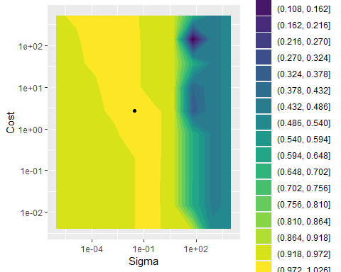
Testing predictive performance
After having tuned the hyperparameters, we can use all data that was
used during the hyperparameter tuning (thus: all folds with training and
validation data) to fit the final model (with the selected
hyperparameter values). For this we can use the
finalize_model function to update the model-specification
with these best hyperparameters:
svm_final <- svm_spec %>%
  finalize_model(svm_best)
Likewise, we can update the workflow by updating the finalized model:
svm_wf_final <- svm_wf %>%
  update_model(svm_final)
We can check the steps above by inspecting the updated final workflow:
svm_wf_final## ══ Workflow ════════════════════════════════════════════════════════════════════════════════════════════════════════════════════════════════════════════════════════
## Preprocessor: Recipe
## Model: svm_rbf()
##
## ── Preprocessor ────────────────────────────────────────────────────────────────────────────────────────────────────────────────────────────────────────────────────
## 1 Recipe Step
##
## • step_normalize()
##
## ── Model ───────────────────────────────────────────────────────────────────────────────────────────────────────────────────────────────────────────────────────────
## Radial Basis Function Support Vector Machine Model Specification (classification)
##
## Main Arguments:
## cost = 2.72158000034875
## rbf_sigma = 0.0278255940220713
##
## Computational engine: kernlabTo perform a last fit of the model based on all training data, and
predict on the testing data (that has not been used during any model
development), we can then use the last_fit function:
svm_final_fit <- svm_wf_final %>%
  last_fit(main_split)
We can compute predictive performance metrics (thus: on the test
dataset) using the collect_metrics function:
svm_final_fit %>%
  collect_metrics()
## # A tibble: 3 × 4
## .metric .estimator .estimate .config
## <chr> <chr> <dbl> <chr>
## 1 accuracy binary 0.96 pre0_mod0_post0
## 2 roc_auc binary 0.994 pre0_mod0_post0
## 3 brier_class binary 0.0286 pre0_mod0_post0Using the collect_predictions function we can retrieve
the predictions on the test dataset, and from this we can then retrieve
the confusion matrix:
svm_final_fit %>%
  collect_predictions() %>%
  conf_mat(truth = Species,
           estimate = .pred_class)
## Truth
## Prediction versicolor virginica
## versicolor 12 0
## virginica 1 12We see that the test dataset contains 25 records (25% of the 100 records we started with). The model fitted and tuned on the other 75% of the data predicts quite well on this test dataset: of the 25 records, 24 were correctly classified (96% accuracy)!