Initial state variables

Ideally, we define a function, let’s call it InitLogistic, that returns a named vector with initial state values:

InitLogistic <- function(N = 5) {
  # Gather function arguments in a named vector
  y <- c(N = N)
  
  # Return the named vector
  return(y)
}

After defining the function, we can retrieve the initial state values (at their defaults), simply using:

InitLogistic()

## N 
## 5

But, we can also retrieve the initial states while changing values compared to their defaults, e.g.:

InitLogistic(N = 6)

## N 
## 6

The here-described way of defining a named vector with initial state values via first defining a function and then calling the function may at first seem like an inefficient method. However, when models become more complex (as they often are), this extra effort easily pays off during simulation and scenario testing.

Parameter values

In a similar way, we can define a function, let’s call it ParmsLogistic, that returns a named vector with parameter values. Parameters and their default values can be specified in the function arguments, so that we can call the function without having to specify their value every time, yet still have the possibility to give them a specific value. For some parameters, it may be sufficient to specify them within the function body, e.g., when there are parameters that will have a fixed value throughout all model analyses and are thus not going to be changed.

ParmsLogistic <- function(r = 0.3, # intrinsic population growth rate
                          K = 100  # carrying capacity
                          ) {
  # Gather function arguments in a named vector
  y <- c(r = r,
         K = K)
  
  # Return the named vector
  return(y)
}

Now, in a similar fashion as above, we can retrieve the parameters, at their default values, simply using:

ParmsLogistic()

##     r     K 
##   0.3 100.0

Alternatively, we can retrieve the parameters at their default values while changing the value of a/some specified parameter(s) simply by passing the value to the respective function argument(s):

ParmsLogistic(r = 0.5)

##     r     K 
##   0.5 100.0

Rates of change

Now we can specify a function that calculates the rates of change of the state variables with respect to time. Let’s call the function RatesLogistic. Check the documentation of the ode function, ?ode(), to see the requirements that the function RatesLogistic should adhere to. Notably, the inputs to the function should be: t, y, parms, in that order (although we can call them differently)! Also, pay attention to the way the function should return its output! As the help-file of the ode function states, the data returned should be a list, where the first element is a vector with the rates of change (in the same order as y!), and all other elements are (optional) extra output, which should be named.

In the example below, we let the function return the rate of change of $N$ (thus $\frac{dN}{dt}$) in 2 places: both in the first element of the returned list (thus used by the ode function for the numerical integration), but also in the optional extra list elements (which should be named and which will be included in the output for each specific time point). By doing so, we not only numerically integrate the dynamics of population $N$, but also keep track of the rate of change of $N$ at the specified time points.

RatesLogistic <- function(t, y, parms) {
  # use the with() function to be able to access the parameters and states easily
  # remember that the with() function is with(data, expr), where
  # - 'data' is ideally a list with named elements
  #   thus: 'y' and 'parms' are combined using function c and converted using function as.list
  # - 'expr' is an expression (i.e. code) that is evaluated
  #   this can span multiple lines of code when embraced with curly brackets {}
  with(
    as.list(c(y, parms)),{
      
      # Optional: forcing functions: get value of the driving variables at time t (if any)
      # see template 2
      
      # Optional: auxiliary equations

      # Rate equations
      dNdt <- r*N*(1-N/K)
      
      # Gather all rates of change in a vector
      # - the rates should be in the same order as the states (as specified in 'y')
      # - it can be a named vector, but does not need to be
      RATES <- c(dNdt = dNdt)
      
      # Optional: get in/out flow used to compute mass balances (or set MB <- NULL)
      # see template 4
      MB <- NULL

      # Optional: gather auxiliary variables that should be returned (or set AUX <- NULL)
      # - this should be a named vector or list!
      # here we pass the rate of change of N with respect to time back as auxiliary variable
      AUX <- RATES 
      
      # Return result as a list
      # - the first element is a vector with the rates of change (in the same order as 'y')
      # - all other elements are (optional) extra output, which should be named
      outList <- list(c(RATES, # the rates of change of the state variables
                        MB),   # the rates of change of the mass balance terms if MB is not NULL
                      AUX) # optional additional output per time step
      return(outList)
    }
  )
}

Solving the model

After installing and loading the deSolve, we can solve the model numerically using the ode() function. We can check the use of this function using ?ode(), where we see that there are (at least) 4 function arguments that need our input:

• y: the initial state values, a vector. If it has named elements, these names will be used to label the output matrix;
• times: time sequence for which output is wanted; the first value of times is the initial time;
• func: a function that computes the values of the derivatives at time t,
• parms: parameters of the model passed to func.

Input for the function argument y can be generated using the above-defined function InitLogistic. Likewise, input for the function argument parms can be generated using the above-defined function ParmsLogistic. Input for the function argument times still needs to be defined, here let’s solve the model for times from 0 (the initial time) to 50 with increments of 1. For this we can simply use the short-hand code 0:50, but also the more versatile code seq(from=0, to=50, by=1) (more versatile because we can easily choose another time-step!). Input for the function argument func is the function RatesLogistic as defined above. Note that we pass the entire function RatesLogistic to this argument, and do not evaluate the function, thus we do not pass RatesLogistic() as input to the func argument, but RatesLogistic! Below, we also pass a value to the method argument to specify that we want to use an adaptive stepsize Runge-Kutta integration method: “ode45”).

states <- ode(y = InitLogistic(),
              times = seq(from = 0, to = 50, by = 1),
              func = RatesLogistic,
              parms = ParmsLogistic(),
              method = "ode45")

Exploring the solved model

The object states now contains the solved model: it is a matrix of class deSolve (see the Value slot in the ?ode() function documentation):

class(states)

## [1] "deSolve" "matrix"

To explore the object states, we can thus look at the top (header; using the head function) and bottom (tail; using the tail function) rows of the matrix, and use the defaults plotting method (using the function plot) to plot the solved model:

head(states)

##      time         N     dNdt
## [1,]    0  5.000000 1.425000
## [2,]    1  6.633260 1.857977
## [3,]    2  8.750883 2.395531
## [4,]    3 11.461553 3.044364
## [5,]    4 14.875003 3.798704
## [6,]    5 19.085896 4.632955

tail(states)

##       time        N         dNdt
## [46,]   45 99.99740 0.0007814116
## [47,]   46 99.99807 0.0005788920
## [48,]   47 99.99857 0.0004288582
## [49,]   48 99.99894 0.0003177084
## [50,]   49 99.99922 0.0002353655
## [51,]   50 99.99942 0.0001743638

plot(states)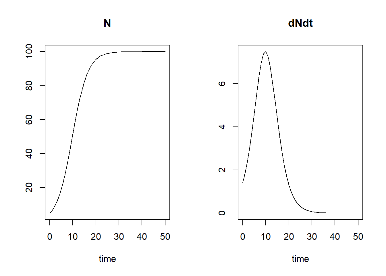

The first column of states is called “time”, with the values corresponding to what we supplied to the function argument times when calling the ode function. The second column is called “N”: this is because the InitLogistic function that we used to pass the initial state value to the argument y returns a vector with the name “N”, so this is the population size. The third and last column is called “dNdt”: this is the optional auxiliary data that we chose to also return. The default plotting method will plot how the state variables, as well as the returned auxiliary variables, evolve over time.

Note that at time 0, $N=5$ (our set initial value!) and $\frac{dN}{dt}=1.425$. But note that at time 1, the value of $N$ is not equal to $5+1.425=6.425$! Thus, the numerical integration performed by the ode function used integration timesteps smaller than 1 time unit, while recording the output at the times specified in the times argument (we used here the adaptive stepsize Runge-Kutta integration method: “ode45”). Thus, when using a variable timestep integration methods, input to the times argument effectively specifies the maximum timestep that will be used in the integration. You can check for yourself whether the value of $N$ at time 1 will be $5+1.425=6.425$ when using Euler integration (use method="euler").

Now, suppose that we want to know the value of $N$ at time 50, we have a few options to retrieve this. First, we can simply read out the value from the corresponding row, e.g. using the tail function as used above (here with the extra function argument n=1 to retrieve only the last record):

tail(states, n = 1)

##       time        N         dNdt
## [51,]   50 99.99942 0.0001743638

Alternatively, we can use the subset function:

subset(states, time == 50)

##            N         dNdt 
## 9.999942e+01 1.743638e-04

Or, we could use matrix indexing using the square bracket notation [,] to retrieve either the 51th row explicitly (i.e. the row corresponding to time 50), or the last row of the matrix (using the function nrow):

states[51,]

##         time            N         dNdt 
## 5.000000e+01 9.999942e+01 1.743638e-04

states[nrow(states),]

##         time            N         dNdt 
## 5.000000e+01 9.999942e+01 1.743638e-04

What we see here, also from the graph above, is that the population $N$ has almost reached a value of 100 at time 50, i.e. it is very close to its carrying capacity $K=100$!

Because we returned the rate of change also as an auxiliary variable, we can now plot how $\frac{dN}{dt}$ varies with $N$:

plot(states[,"N"], states[,"dNdt"], type = "l", xlab = "N", ylab = "dN/dt")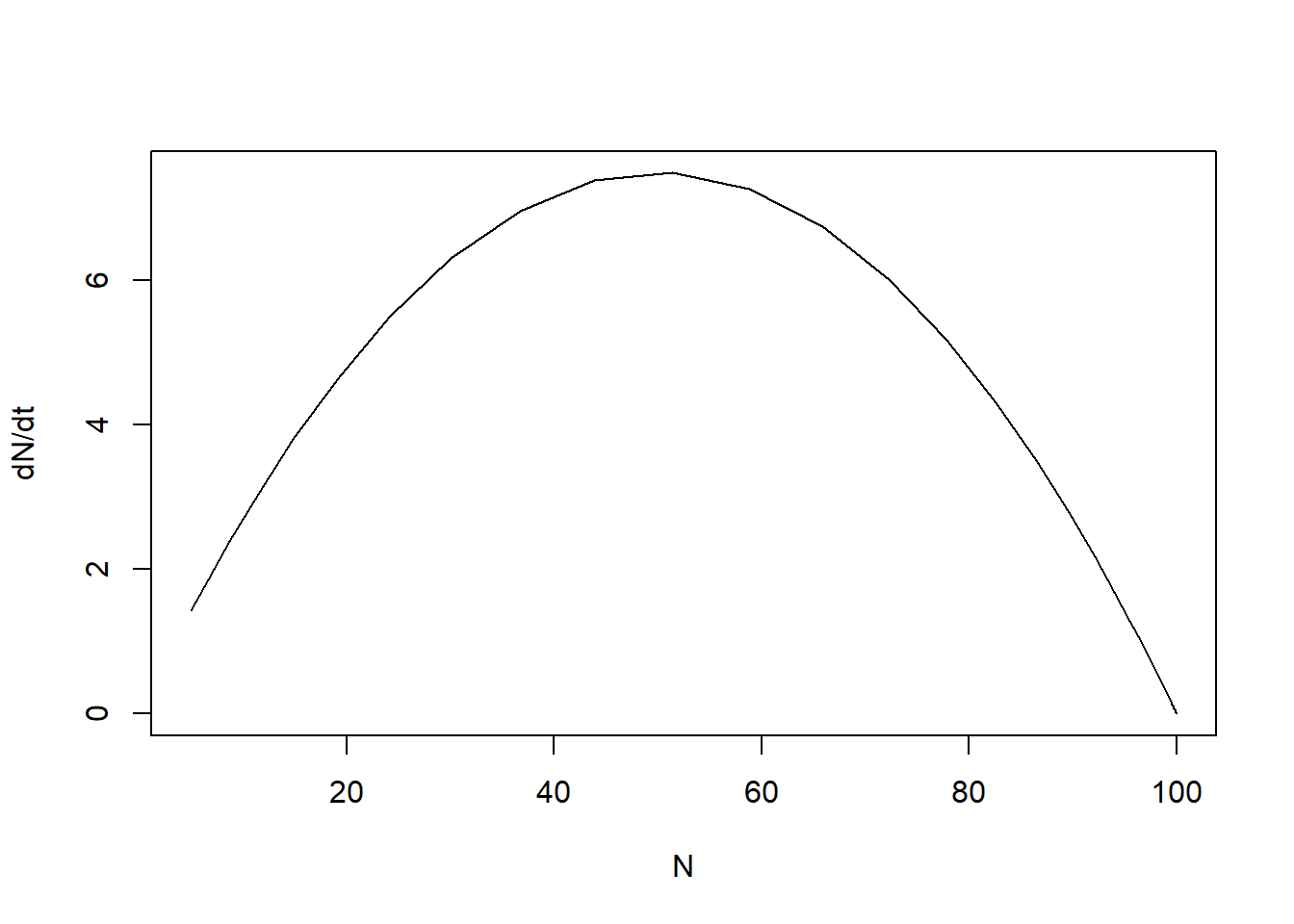

Downloadable R script

An R script with the code chunks of the above example can be downloaded here.