Wageningen University & Research | FEM-31806 | Models for Ecological Systems | FEM | PPS | WEC
CO2Fix - Day 4
First make a copy of the script you created on Day 2 to implemented the model (or, copy the solution of the implementation of the model from the solution to day 2, and then continue with the exercises below.
Aims
Aim 1: Sensitivity
Probably you have already separated parameters between those that are true constants (e.g. molar weights, physical properties etc.), those that are more or less invariable or are measured with great precision and therefore hard coded in the parameter list, and those that are highly uncertain and/or can vary a lot in different scenarios. The latter are in this course typically defined per scenario and given as input arguments to the function creating a named vector with parameter values, or as a defined list in input scenario-specific input files for other models.
Select three parameters for sensitivity analysis. Run both a sensitivity analysis (sensu stricto), and also an elasticity analysis, which is a normalized version of sensitivity (see textbook and lectures for differences). Run the model three times (50 years) but with different parameter values: at the default parameter value, at the default parameter value -10%, and at the default parameter value +10%. Study the effects of these parameter values for the state variables: Wc reflecting the total amount of carbon (Wc = Wf + Ws + Wr + Wp + Wt + Ww). Visualize by plotting the results. For visualization you can first best plot the state variable(s) of interest against time (possibly with multiple scenarios in a single plot; a separate line for each scenario). Moreover, you can opt for a barplot showing the sensitivity and elasticity index values for the parameters.
Aim 2: Calibration
- Calibrate the model for three critical and uncertain parameters: cdgs, nf and rgt. Use the data sets provided on Brightspace (CO2Fix.csv). Calibrate the model for state variable WS, using the numerical optimization method as developed in Template 6. Visualize the implications for the model: plot the state variables against time.
Aim 3: Validation
Give the options to validate your model.
What data would you need?
Answers
Download here the code as shown on this page in a separate .r file.
Sensitivity
Parameters
The function returning a named vector with parameter values:
ParmsCO2fix <- function(
      ### External conditions
      IE = 200.0,  # IE external light intensity. If we consider the value of 200 and its
      # units of J PAR / (m2 s), this means for a day-length of 12 hours
      # 8.64 MJ / (m2 d). This is a reasonable value as an average over a
      # season, but the highest values during days of the season may reach
      # 30 MJ / (m2 d) or even more.
      CDGS = 200,  # CDGS days in a growing season, d/season, which is effectively d/y.
      CDLH = 12,   # CDLH sun hours in a day, hour/day = h/d.

      ### Tree specific parameters
      K = 0.7,     # K Light extinction coefficient (ranges from 0.5 - 0.9) m2 soil / (m2 leaf)
      SLA = 15.0,  # Specific Leaf Area (ranges from 10 - 20) m2 leaf / (kg leaf)
      FCL = 0.5,   # Fraction of C per mass of leaf: kgC / (kg of Leaf)
      LUE = 1.E-8, # Light use efficiency (ranges from 1.(08) - 4.3(2) gDW/MJ or
      # 0.001- 0.0043 kgDW/MJ), Sinclair and Muchow, 1999).
      # However, since the unit is here given in kg CO2 / (J PAR), the
      # range is between 1.8E-9 - 7.9E-9. The LUE is taken as 1.E-8,
      # which appears rather high.
      # Photosynthesis (PG), etc. are in terms of C(arbon), and the LUE should
      # also be given in gC/MJ. Assuming 50% of C per gram of dry matter
      # (DW) this would mean a value between 0.5 * (0.001- 0.0043 kgDW/MJ)
      # = 0.0005 - 0.0022 kgC/MJ.
      CF = 0.9,    # CF dimensionless curvature factor of the NRH or photosynthesis curve.
      PC = 1.E-6,  # PC photosynthesis capacity in kg CO2/(m2 s).

      # Allocation fractions: (kg assimilates to organ)/(kg assimilates produced by photosynthesis)
      NF = 0.2,      # constant allocation fraction of assimilates to foliage
      NS = 0.6,      # constant allocation fraction of assimilates to stem
      NR = 1 - (NF + NS), # The fraction to roots: 1 - fraction to (foliage+stem)

      # RF, RR and RS are (carbon) mass-based relative respiration rates for
      # F (foliage), R (roots) and S (shoot). Unit 1/year.
      RF = 0.1,
      RR = 0.1,
      RS = 0.1,
      # relative death rates or turnover rates, for
      # F (foliage), R (Roots), S (stem), and transition from sapwood to heartwood Unit 1/year.
      LRF = 1.0,
      LRR = 0.2,
      LRS = 0.05, # equal for sapwood and heartwood
      TSH = 0.1,

      ### Management related parameters
      NH = 0.1, # NH relative harvesting rate, 1/year, NP and NT: constant allocation
      # Unit NP       ; unit NT
      # (kgC of paper) (kgC of timber wood)
      # ------------- --------------------
      # (kgC of wood) (kgC of wood)
      NP = 0.2,   # fractions of harvested product to paper, NP, and timber, NT.
      NT = 1 - NP,# fractions of harvested product to timber
      LRP = 0.5,  # relative decay rates or turnover rates, for
      LRT = 0.02, # P (Paper) and T (Timber). Unit 1/year.
      LRW = 0.1   # loss rate waste
      # The inverse of these numbers gives the average residence time of the
      # product. If RGT=0.02, this means an average residence time of 50 years.
  ){

  # Constants, such as molecular weights. Constants must not be changed.
  MWC <- 12 # molar weight of C, g/mol
  MWO <- 16 # molar weight of O, g/mol
  # number of seconds per hour
  CSPH <- 3600

  # Gather parameters in a named vector
  y <- c(IE = IE, CDGS = CDGS, CDLH = CDLH, K = K, SLA = SLA,
         FCL = FCL, LUE = LUE, CF = CF, PC = PC,
         NF = NF, NS = NS, NR = NR,
         RF = RF, RR = RR, RS = RS, LRF = LRF, LRR = LRR, LRS = LRS, TSH = TSH,
         NH = NH, NP = NP, NT = NT, LRP = LRP, LRT = LRT, LRW = LRW,
         MWC = MWC, MWO = MWO, CSPH = CSPH)

  # Return
  return(y)
}
Initial conditions
The function returning a named vector with initial state values (all in units kgC m-2), here initialization according to the fractions that are allocated to the organs during the simulation:
InitCO2fix <- function(WF = 0.02, # WF, kgC in Foliage/m2
                       WR = 0.02, # WR, kgC in Roots/m2
                       WS = 0.06, # WS, kgC in Stems/m2
                       WH = 0.0,  # WH, kgC in Stems/m2
                       WP = 0.0,  # WP  kgC in paper/ m2
                       WT = 0.0,  # WT, kgC in timber/m2
                       WW = 0.0   # WW, kgC in waste/m2
                       ){
  # Gather initial conditions in a named vector; given names are names for the state variables in the model
  y <- c(WF = WF,
         WR = WR,
         WS = WS,
         WH = WH,
         WP = WP,
         WT = WT,
         WW = WW)

  # Return
  return(y)
}
Differential equations
The function computing the rates of change of the state variables with respect to time:
RatesCO2fix <- function(t, y, parms) {
  # use the with() function to be able to access the parameters and states easily
  # remember that the with() function is with(data, expr), where
  # - 'data' is ideally a list with named elements
  #   (thus combine 'y' and 'parms' first, using the function c(), then convert to list using as.list())
  # - 'expr' is an expression (i.e. code) that is evaluated
  #   this can span multiple lines of code when embraced with curly brackets {}
  with(
    as.list(c(y, parms)),{

      ### Optional: forcing functions: get value of the driving variables at time t (if any)

      ### Optional: auxiliary equations
      LAI <- WF * SLA / FCL
      IA <- IE *(1 - exp(-K * LAI ))

      PGS <- (1 / (2 * CF)) * (LUE * IA + PC -
                                 sqrt((LUE * IA + PC)^2 -4 * CF * LUE * IA* PC) )
      PG <- PGS * CSPH * CDLH * CDGS * (MWC / (MWC + 2 * MWO))
      PN <- PG - (RF * WF + RR * WR + RS * WS)

      ### Rate equations
      DWFDT <- PN * NF - LRF * WF - NH * WF
      DWRDT <- PN * NR - LRR * WR - NH * WR
      DWSDT <- PN * NS - LRS * WS - NH * WS - TSH*WS
      DWHDT <- TSH* WS - LRS * WH - NH * WH

      HT <- NH * (WF + WR + WS + WH) # total harvest
      HU <- NH * (WS + WH)           # useful harvest

      # The useful harvest, HU, is only the stem, so: (NH*DWS).
      # This is distributed over the two states paper and timber. These are
      # fractions of the useful harvest: paper NP; timber NT=(1-NP).
      DWPDT <- HU * NP - LRP * WP # paper
      DWTDT <- HU * NT - LRT * WT # Timber
      DWWDT <- HT - HU + LRF * WF + LRR * WR +LRS *(WS+WH) - LRW * WW # Waste

      ### Gather all rates of change in a vector
      # - the rates should be in the same order as the states (as specified in 'y')
      # - it can be a named vector, but does not need to be
      RATES <- c(DWFDT = DWFDT,
                 DWRDT = DWRDT,
                 DWSDT = DWSDT,
                 DWHDT = DWHDT,
                 DWPDT = DWPDT,
                 DWTDT = DWTDT,
                 DWWDT = DWWDT)

      ### Optional: get in/out flow used to compute mass balances (or set MB <- NULL)
      # not included here (thus here use MB <- NULL), see template 3
      MB <- NULL

      ### Optional: gather auxiliary variables that should be returned (or set AUX <- NULL)
      # - this should be a named vector or list!
      AUX <- NULL

      # Return result as a list
      # - the first element is a vector with the rates of change (in the same order as 'y')
      # - all other elements are (optional) extra output, which should be named
      outList <- list(c(RATES, # the rates of change of the state variables (same order as 'y'!)
                        MB),   # the rates of change of the mass balance terms (or NULL)
                      AUX) # optional additional output per time step
      return(outList)
    })
}
With these 3 functions now defined, the CO2Fix mini-model has been
implemented in R code, and the model can now numerically be solved using
the ode function from the deSolve package.
Here, let’s solve the model for 3 different values of parameter
CDGS: first for its default value (200; solved model stored
in states), then when increasing it by 10% (solved model
stored in statesHI), and then when decreasing it with 10%
(solved model stored in statesLO).
states <- ode(y = InitCO2fix(),
              times = seq(from = 0, to = 50, by = 1),
              func = RatesCO2fix,
              parms = ParmsCO2fix(CDGS = 200),
              method = "ode45")
statesHI <- ode(y = InitCO2fix(),
                times = seq(from = 0, to = 50, by = 1),
                func = RatesCO2fix,
                parms = ParmsCO2fix(CDGS = 1.1*200),
                method = "ode45")
statesLO <- ode(y = InitCO2fix(),
                times = seq(from = 0, to = 50, by = 1),
                func = RatesCO2fix,
                parms = ParmsCO2fix(CDGS = 0.9*200),
                method = "ode45")
We can show these different scenarios:
plot(states, statesHI, statesLO)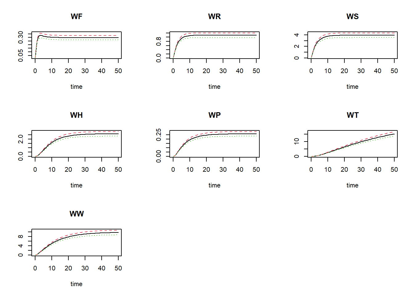
where the black line is the default value for CDGS, the
red line is the high value (10% increase), and the green line shows the
simulation for the value reduced by 10%.
We can now calculate the sensitivity index (SI) and elasticity index
(EI) of the parameter CDGS on state total carbon (Wf + Ws +
Wr + Wp + Wt + Ww) at the end of the simulation:
carbonColumns <- c("WF", "WS", "WR", "WP", "WT", "WW")
deltaState <- sum(statesHI[nrow(statesHI),carbonColumns]) - sum(statesLO[nrow(statesLO),carbonColumns])
deltaParm <- 0.1*200
SI <- deltaState / (2*deltaParm)
SI
## [1] 0.1532905EI <- (deltaState/sum(states[nrow(states),carbonColumns])) / ((2*deltaParm) / 200)
EI## [1] 1.00145This approach can be repeated for the other parameters and both state variables. Repeating the same procedure for all parameters and all state variables yields the following elasticity indices:
# Get initial conditions, parameters and the simulation output times
inits <- InitCO2fix()
parms <- ParmsCO2fix()
times <- seq(from = 0, to = 50, by = 1)

# Create empty vectors to hold the differences in the state variable (stateDiff) and parameters (parmDiff)
stateDiff <- parms # this makes of copy of the named parameter vector
parmDiff  <- parms
stateDiff[] <- NA # This sets all elements within the vector to value NA
parmDiff[] <- NA
# the result is 2 empty (values: NA) named numeric vectors (with the names of the parameters)

# Set the fraction by which each parameter is decreased/increased during sensitivity analysis
changeFraction <- 0.1 # 10%

# Set the time at which we want to evaluate the values of the state variables (a value that occurs in 'times'!)
evalTime <- max(times) # we use the last time in the output, but it can be other times as well

# In a 'for'-loop with iterator "i":
# - create 2 copies of 'parms': called 'parmsLo' and 'parmsHi'
# - reduce the value of the i-th parameter in parmsLo with 'changeFraction'
# - increase the value of the i-th parameter in parmsHi with 'changeFraction'
# - solve the ODE model for both parameter sets (they are identical except for the i-th parameter)
# - retrieve the values of the state 'stateName' after 'evalTime' time units and store the difference in 'stateDiff'
# - store the difference between the elevated and reduced parameter value in 'parmDiff'
for(i in seq_along(parms)){
  # create copies of parms
  parmsLo <- parms
  parmsHi <- parms

  # Reduce/increase the value of the i-th parameter
  parmsLo[[i]] = (1 - changeFraction) * parms[[i]]
  parmsHi[[i]] = (1 + changeFraction) * parms[[i]]

  # Solve the ODE model for both sets of parameters
  states_lo <- ode(y = inits,
                   times = times,
                   parms = parmsLo,
                   func = RatesCO2fix,
                   method = "ode45")
  states_hi <- ode(y = inits,
                   times = times,
                   parms = parmsHi,
                   func = RatesCO2fix,
                   method = "ode45")

  # Retrieve the values of the state variable after evalTime time units and store as the i-th element in stateDiff
  states_hi <- subset(states_hi, time==evalTime)
  states_lo <- subset(states_lo, time==evalTime)
  stateDiff[[i]] <- sum(states_hi[carbonColumns]) - sum(states_lo[carbonColumns])

  # Store the difference between the elevated and reduced parameter value in the i-th element of parmDiff
  parmDiff[[i]] <- parmsHi[[i]] - parmsLo[[i]]
}
We can now compute the sensitivity index:
SI <- stateDiff / parmDiff
round(SI, 5)
## IE CDGS CDLH K SLA FCL LUE CF PC NF NS
## 2.003000e-02 1.532900e-01 2.554840e+00 8.990000e-02 4.200000e-03 -1.202800e-01 4.005913e+08 2.195191e+01 2.670798e+07 1.594245e+01 2.883252e+01
## NR RF RR RS LRF LRR LRS TSH NH NP NT
## 1.413560e+01 -4.209980e+00 -1.513376e+01 -5.417006e+01 6.896000e-02 1.307830e+00 -4.405809e+01 5.137620e+00 4.870975e+01 1.309810e+00 1.913173e+01
## LRP LRT LRW MWC MWO CSPH
## -5.290700e-01 -2.922817e+02 -9.355903e+01 1.859430e+00 -1.400880e+00 8.520000e-03We can also calculate the elasticity indices, here rounded to 5 digits and sorted on decreasing absolute value:
states <- ode(y = inits,
                  times = times,
                  parms = parms,
                  func = RatesCO2fix,
                  method = "ode45")
Es <- parms / sum(states[nrow(states),carbonColumns]) * SI
round(Es[order(abs(Es),decreasing=TRUE)],5)
## CSPH CDLH CDGS PC MWO MWC CF NS NT LRW LRT RS NH LUE IE NF NR
## 1.00145 1.00145 1.00145 0.87242 -0.73216 0.72886 0.64536 0.56509 0.49995 -0.30561 -0.19095 -0.17695 0.15911 0.13085 0.13085 0.10415 0.09235
## LRS RR TSH RF LRP NP LRR LRF K SLA FCL
## -0.07196 -0.04943 0.01678 -0.01375 -0.00864 0.00856 0.00854 0.00225 0.00206 0.00206 -0.00196We could use a barplot to show the elasticities:
barplot(Es, col = 1:8, beside = TRUE)
legend(x = "topright", horiz = FALSE, bty = "n", legend = names(Es), pch = 22, cex = 0.7, col = 1:8)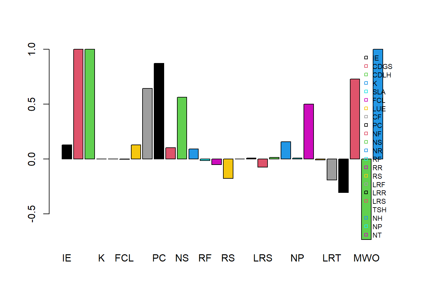
Calibration
First, load the data from the file CO2fix.csv, omitting the first 2 rows (names, and units), after which we assign the names manually:
dat = read.table("pathToFileFolder/CO2fix.csv", head=FALSE, sep=',', skip=2)
names(dat) = c("time","WS","Ctot")
Explore the data by showing the header of the file:
head(dat)## time WS Ctot
## 1 5 4.9545 7.8454
## 2 8 6.1666 10.7690
## 3 14 7.0644 15.1360
## 4 20 7.2914 18.5880
## 5 22 7.3200 19.6150
## 6 27 7.3540 21.9760Let’s first simulate the model with default parameter and initial state values, and check how well the modelled predictions for “V” agree with the measured values for state “V”:
# Simulate with default parameter values
states <- ode(y = InitCO2fix(),
              times = seq(from = 0, to = 50, by = 1),
              parms = ParmsCO2fix(),
              func = RatesCO2fix,
              method = "ode45")
# Plot
plot(states[,"time"], states[,"WS"], type="l", xlab="Time", ylab="WS", ylim=c(0,7.5))
points(dat$time, dat$WS, pch=16)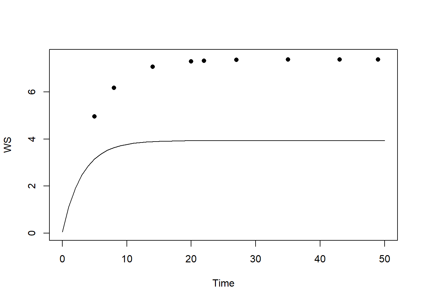
We see that the model systematically underestimates the value of WS.
In order to calibrate the model, we first have to define a few
functions (predictionError, predRMSE,
transformParameters and calibrateParameters)
that allow us to do the calibration. These functions can be found in
template 6. Note that we do not have to fill something in here: we only
are defining these functions as is, and later when we
call (use) these functions we have to supply them with the
appropriate inputs.
First, function predictionError (copy from template
6):
# Define a function that computes prediction errors
# NOTE: nothing needs to be filled in here, so this function can be used as-is
# (unless there is a need to change it, e.g. change the solver method, or include events etc.)
predictionError <- function(p,          # the parameters
                            y0,         # the initial conditions
                            fn,         # the function with rate equation(s)
                            name,       # the name of the state parameter
                            obs_values, # the measured state values
                            obs_times,  # the time-points of the measured state values
                            out_time = seq(from = 0, # times for the numerical integration
                                           to = max(obs_times), # default: 0 - max(obs_times)
                                           by = 1) # in steps of 1
                            ) {
  # Get out_time vector to retrieve predictions for (combining 'obs_times' and 'out_time')
  out_time <- unique(sort(c(obs_times, out_time)))

  # Solve the model to get the prediction
  pred <- ode(y = y0,
              times = out_time,
              func = fn,
              parms = p,
              method = "ode45")
  # NOTE: in case of a 'stiff' problem, method "ode45" might result in an error that the max nr of
  # iterations is reached. Using method "rk4" (fixed timestep 4th order Runge-Kutta) might solve this.

  # Get predictions for our specific state, at times t
  pred_t <- subset(pred, time %in% obs_times, select = name)

  # Compute errors, err: prediction - obs
  err <- pred_t - obs_values

  # Return
  return(err)
}
Note that if Second, function predRMSE (copy from
template 6):
# Define a function that computes the Root Mean Squared Error, RMSE
# NOTE: nothing needs to be filled in here, so this function can be used as-is
predRMSE <- function(...) { # NOTE: these ... are ellipsis, so DO NOT fill in something here!
  # Get prediction errors
  err <- predictionError(...) # NOTE: these ... are ellipsis, so DO NOT fill in something here!

  # Compute the measure of model fit (here the Root Mean Squared Error)
  RMSE <- sqrt(mean(err^2))

  # Return the measure of model fit
  return(RMSE)
}
Third, function transformParameters (copy from template
6):
# Define a function that allows for transformation and back-transformation
# NOTE: nothing needs to be filled in here, so this function can be used as-is
transformParameters <- function(parm, trans, rev = FALSE) {
  # Check transformation vector
  trans <- match.arg(trans, choices = c("none","logit","log"), several.ok = TRUE)

  # Get transformation function per parameter
  if(rev == TRUE) {
    # Back-transform from real scope to parameter scope
    transfun <- sapply(trans, switch,
                       "none" = mean,
                       "logit" = plogis,
                       "log" = exp)
  }else {
    # Transform from parameter scope to real scope
    transfun <- sapply(trans, switch,
                       "none" = mean,
                       "logit" = qlogis,
                       "log" = log)
  }

  # Apply transformation function
  y <- mapply(function(x, f){f(x)}, parm, transfun)

  # Return
  return(y)
}
And fourth, function calibrateParameters (copy from
template 6):
# Define a function that performs the calibration of specified parameters
# NOTE: nothing needs to be filled in here, so this function can be used as-is
calibrateParameters <- function(par,  # parameters
                                init, # initial state values
                                fun,  # function that returns the rates of change
                                stateCol, # name of the state variable
                                obs,  # observed values of the state variable
                                t,    # timepoints of the observed state values
                                calibrateWhich, # names of the parameters to calibrate
                                transformations, # transformation per calibration parameter
                                times = seq(from = 0, # times for the numerical integration
                                            to = max(t), # default: 0 - max(t)
                                            by = 1), # in steps of 1
                                ... # NOTE: these ... are ellipsis, so DO NOT fill in something here!
                                    # these are the optional extra arguments past on to optim()
                                ) {
  # check names of parameters that need calibration
  calibrateWhich <- match.arg(calibrateWhich, choices = names(par), several.ok = TRUE)

  # Create vector with transformations for all parameters (set to "none")
  tranforms <- rep("none", length(par))
  names(tranforms) <- names(par) # set the names of each transformation

  # Overwrite the elements for parameters that need calibration
  tranforms[calibrateWhich] <- transformations

  # Transform parameters
  par <- transformParameters(parm = par, trans = tranforms, rev = FALSE)

  # Get parameters to be estimated
  par_fit <- par[calibrateWhich]

  # Specify the cost function: the function that will be optimized for the parameters to be estimated
  costFunction <- function(parm_optim, parm_all,
                           init, fun, stateCol, obs, t,
                           times = t,
                           optimNames = calibrateWhich,
                           transf = tranforms,
                           ... # NOTE: these ... are ellipsis, so DO NOT fill in something here!
                           ) {
    # Gather parameters (those that are and are not to be estimated)
    par <- parm_all
    par[optimNames] <- parm_optim[optimNames]

    # Back-transform
    par <- transformParameters(parm = par, trans = transf, rev = TRUE)

    # Get RMSE
    y <- predRMSE(p = par, y0 = init, fn = fun,
                  name = stateCol, obs_values = obs, obs_times = t,
                  out_time = times)

    # Return
    return(y)
  }

  # Fit using optim
  fit <- optim(par = par_fit,
               fn =  costFunction,
               parm_all = par,
               init = init,
               fun = fun,
               stateCol = stateCol,
               obs = obs,
               t = t,
               times = times,
               ...) # NOTE: these ... are ellipsis, so DO NOT fill in something here!
                    # These are the optional additional arguments passed on to optim()

  # Gather parameters: all parameters updated with those that are estimated
  y <- par
  y[calibrateWhich] <- fit$par[calibrateWhich]

  # Back-transform
  y <- transformParameters(parm = y, trans = tranforms, rev = TRUE)

  # put all (constant and estimated) parameters back in $par
  fit$par <- y

  # Add the calibrateWhich information
  fit$calibrated <- calibrateWhich

  # return 'fit'object:
  return(fit)
}
After defining these 4 functions, we can get started with the actual calibration. For this we need to make some choices, e.g. which parameters to calibrate, and what are the transformations needed (no transformation, logarithmic transformation, or logit transformation, see explanation in template 6).
Let’s calibrate only the parameters “CDGS” and “NF” of the model,
based on the dataset dat and the measurements (and thus
state) “WS”. We only have to simulate to the maximum time of our dataset
dat (thus max(dat$time)). Parameter “CDGS” can
only be a positive value, so let’s use a log-transform for this
parameter during calibration. Parameter “NF” is a fraction, thus is
bounded between values 0 and 1; thus, let’s use a logit-transform for
this parameter during calibration.
Note that the calibration may take some time (several seconds/minutes) to complete:
# Perform the calibration
fit <- calibrateParameters(par = ParmsCO2fix(),
                           init = InitCO2fix(),
                           fun = RatesCO2fix,
                           stateCol = "WS",
                           obs = dat$WS,
                           t = dat$time,
                           times = seq(from = 0, to = max(dat$time), by = 1),
                           calibrateWhich = c("CDGS","NF"),
                           transformations = c("log","logit"))
We can retrieve information on the model fitting by looking at the
object fit:
fit## $par
## IE CDGS CDLH K SLA FCL LUE CF PC NF NS NR
## 2.000000e+02 3.635007e+02 1.200000e+01 7.000000e-01 1.500000e+01 5.000000e-01 1.000000e-08 9.000000e-01 1.000000e-06 5.203788e-02 6.000000e-01 2.000000e-01
## RF RR RS LRF LRR LRS TSH NH NP NT LRP LRT
## 1.000000e-01 1.000000e-01 1.000000e-01 1.000000e+00 2.000000e-01 5.000000e-02 1.000000e-01 1.000000e-01 2.000000e-01 8.000000e-01 5.000000e-01 2.000000e-02
## LRW MWC MWO CSPH
## 1.000000e-01 1.200000e+01 1.600000e+01 3.600000e+03
##
## $value
## [1] 0.3373857
##
## $counts
## function gradient
## 73 NA
##
## $convergence
## [1] 0
##
## $message
## NULL
##
## $calibrated
## [1] "CDGS" "NF"Explanation of these outputs are given in the explanation section of Template 6:
- “par”: the calibrated parameter values. This includes all model parameters: those that are kept constant as well as those that have been calibrated;
- “value”: this is the value of the cost-function at the values as given in “par”. Here, this is thus the RMSE of the model predictions given the parameter values in “par”;
- “counts”: information about the number of iterations that the
optimfunction needed; - “convergence”: information about the convergence of the
optimfunction: a value of 0 means that the estimation successfully converged! For other values, see?optimfor the help-documentation of theoptimfunction; - “message”: a character string giving any additional information
returned by the optimizer, or
NULL; - “calibrated”: a character string with the model parameters that have
been calibrated (thus the vector passed as input to argument
calibrateWhich).
Then, we can use the fitted/calibrated model parameters (object
fit$par) to simulate the model, and plot the result:
# Fit the model using the calibrated values
statesFitted <- ode(y = InitCO2fix(),
                    times = seq(from = 0, to = 50, by = 1),
                    parms = fit$par,
                    func = RatesCO2fix,
                    method = "ode45")
plot(statesFitted)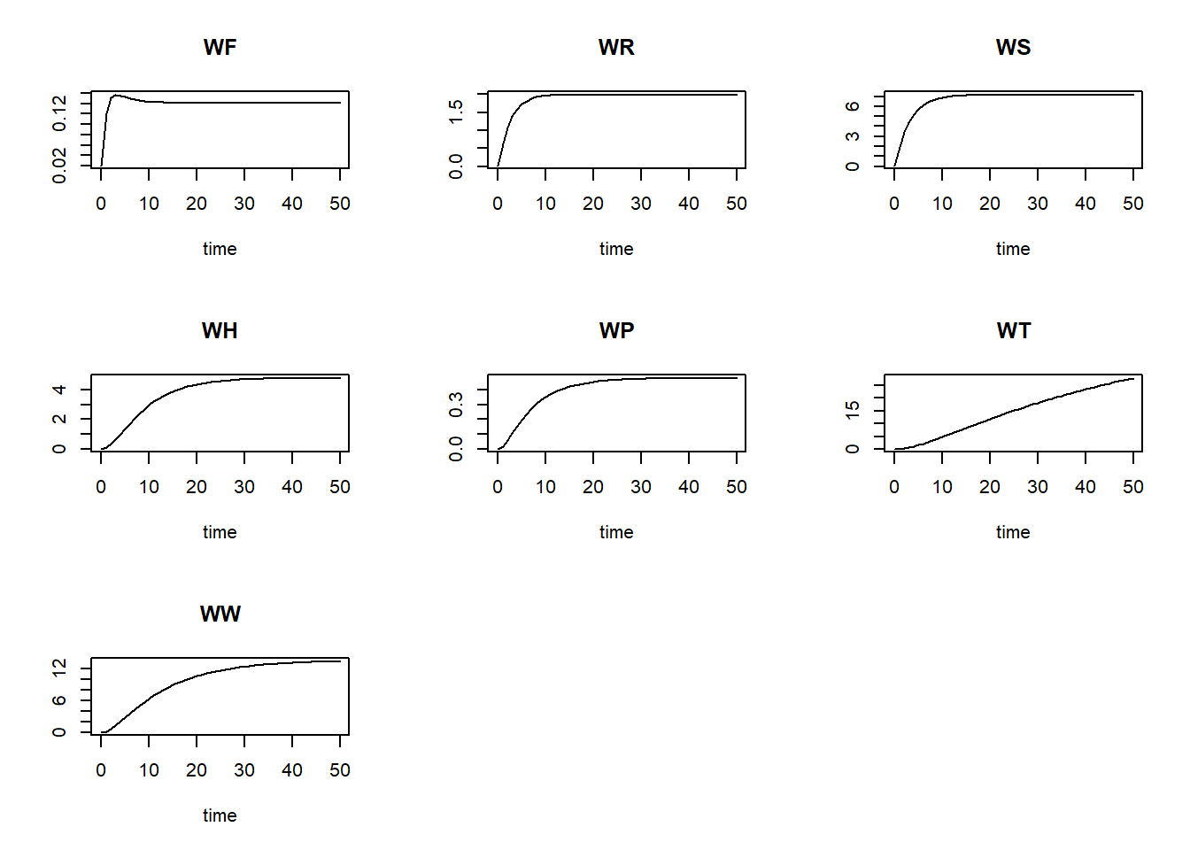
Also, we can plot the modelled pattern of state “WS” as function of time, including the measured values of “WS”:
plot(statesFitted[,"time"], statesFitted[,"WS"], type = "l", xlab = "Time", ylab = "WS")
points(dat$time, dat$WS, pch = 16)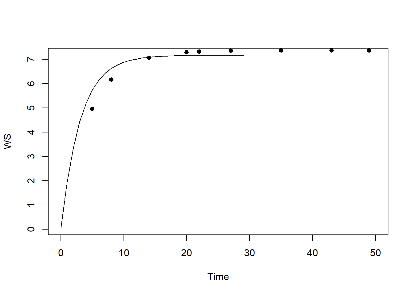
The calibrated model seems to capture the observed pattern quite well! In order to quantify the difference between the calibrated model and the model solved with default parameter values, let’s compute the RMSE for both models:
predRMSE(p = ParmsCO2fix(),
         y0 = InitCO2fix(),
         fn = RatesCO2fix,
         name = "WS",
         obs_values = dat$WS,
         obs_times = dat$time,
         out_time = seq(from = 0, to = 50, by = 1))
## [1] 3.158159predRMSE(p = fit$par,
y0 = InitCO2fix(),
fn = RatesCO2fix,
name = "WS",
obs_values = dat$WS,
obs_times = dat$time,
out_time = seq(from = 0, to = 50, by = 1))## [1] 0.3373857We see that the calibrated model has a RMSE that is much lower than that with the default parameters, thus: via calibration we have improved model fit massively!