Wageningen University & Research | FEM-31806 | Models for Ecological Systems | FEM | PPS | WEC

Here, you will practice some more R skills that will be useful during the coming weeks when we define and analyse models in R:

plotting
for-loops
writing your own functions
using the with function
working with lists to store data

Exercise 3.1

One of the greatest strengths of R, relative to other programming languages, is the ease with which we can create publication-quality graphics. Here, we will try some very basic plotting in R, and do not cover the more advanced ways of plotting using e.g. the lattice, ggplot2 and ggvis libraries.

3.1 a

Have a look at the built-in iris dataset, using the head function

head(iris)

##   Sepal.Length Sepal.Width Petal.Length Petal.Width Species
## 1          5.1         3.5          1.4         0.2  setosa
## 2          4.9         3.0          1.4         0.2  setosa
## 3          4.7         3.2          1.3         0.2  setosa
## 4          4.6         3.1          1.5         0.2  setosa
## 5          5.0         3.6          1.4         0.2  setosa
## 6          5.4         3.9          1.7         0.4  setosa

The default plot function applied to a data.frame will give you a plot where all columns in the data.frame are plotted against each other (i.e., pair plots). Give it a try.

plot(iris)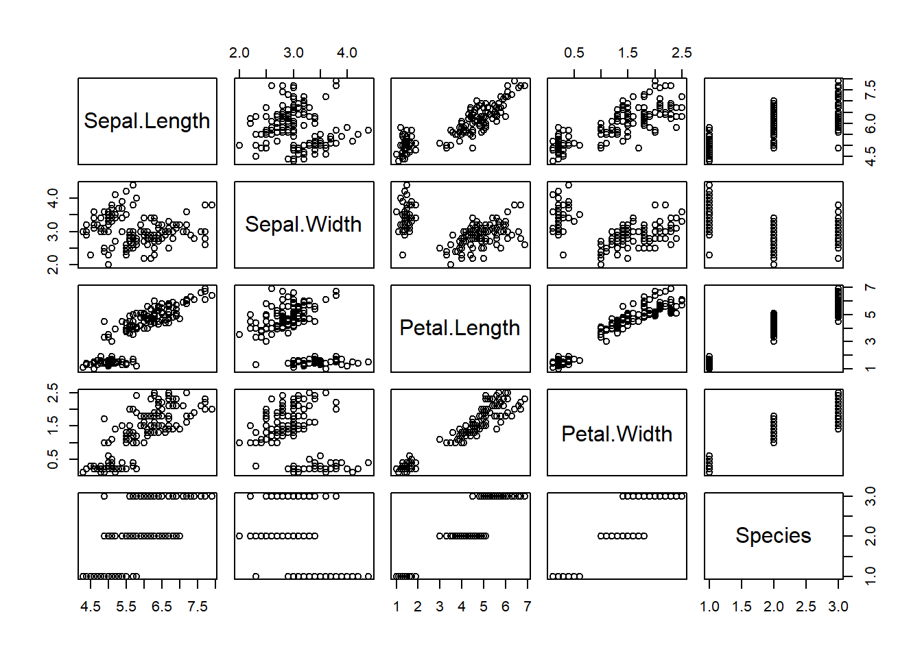

3.1 b

Remember that you can use the $-sign to retrieve entire columns from a data.frame. Plot 2 specific columns against each other the $-sign notation: plot column Sepal.Length on the x-axis and column Sepal.Width on the y-axis.

plot(iris$Sepal.Length, iris$Sepal.Width)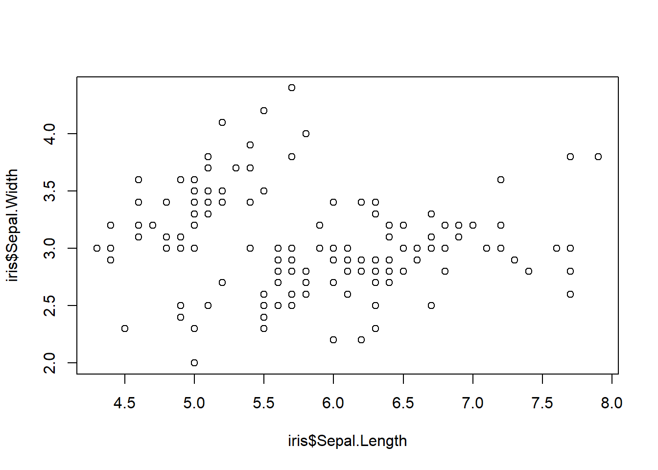

3.1 c

Alternatively, you can use square bracket [] notation to index specific columns from the data.frame (or matrix). Remember that a data.frame is a 2-dimensional data structure, and indexing the column should be done in the second element of the index: e.g. iris[,4] returns the 4^th column in the iris dataset. Create the same plot with column Sepal.Length on the x-axis and column Sepal.Width on the y-axis using [] notation and the column position numbers.

plot(iris[,1], iris[,2])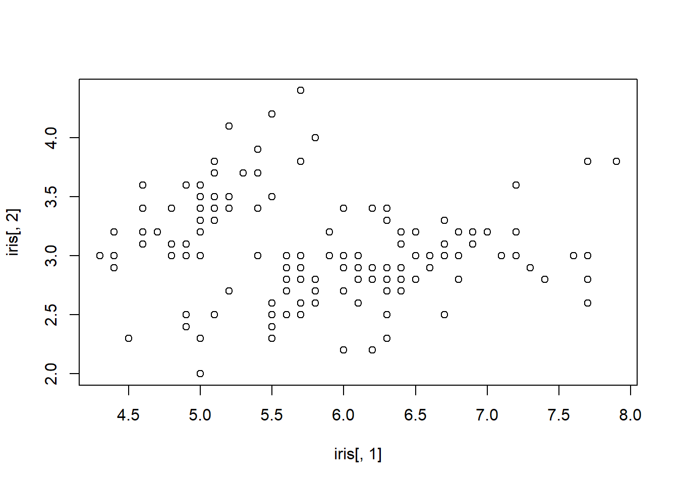

Do the same but now using the column names as character objects.

plot(iris[,"Sepal.Length"], iris[,"Sepal.Width"])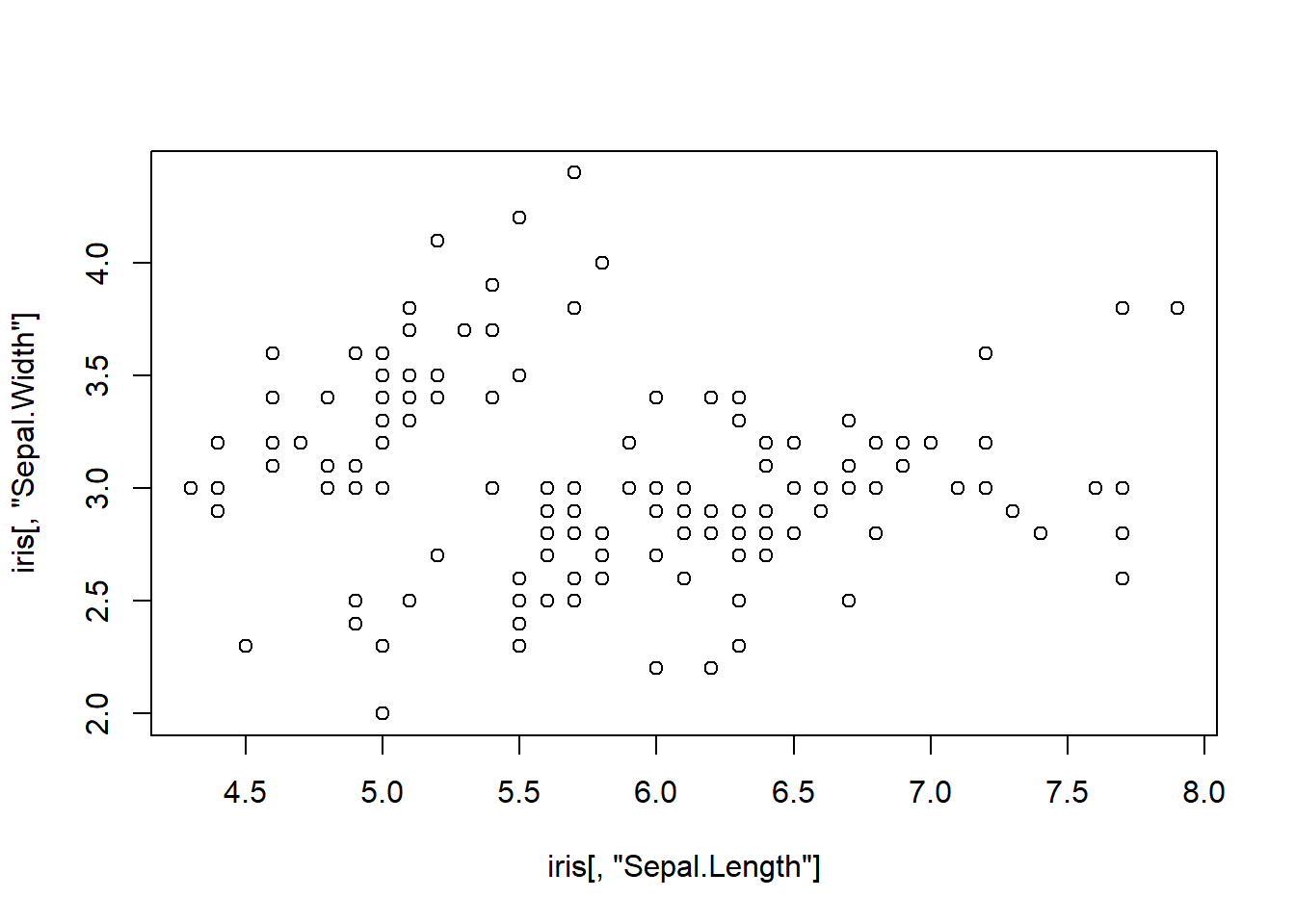

3.1 d

Adjust your plot by adding extra arguments so as to specify that “length” is the x-axis label, “width” the y-axis label, that the point type is 16 and the point colour is green.

To specify the axis labels in a plot() function call, you can use the arguments xlab and ylab for x-axis and y-axis labels, respectively. To specify point type and colour, use function arguements pch and col, respectively.

plot(iris$Sepal.Length, iris$Sepal.Width,
     xlab = "length", # x axis label
     ylab = "width",  # y axis label
     pch = 16, # point type
     col = "green") # point colour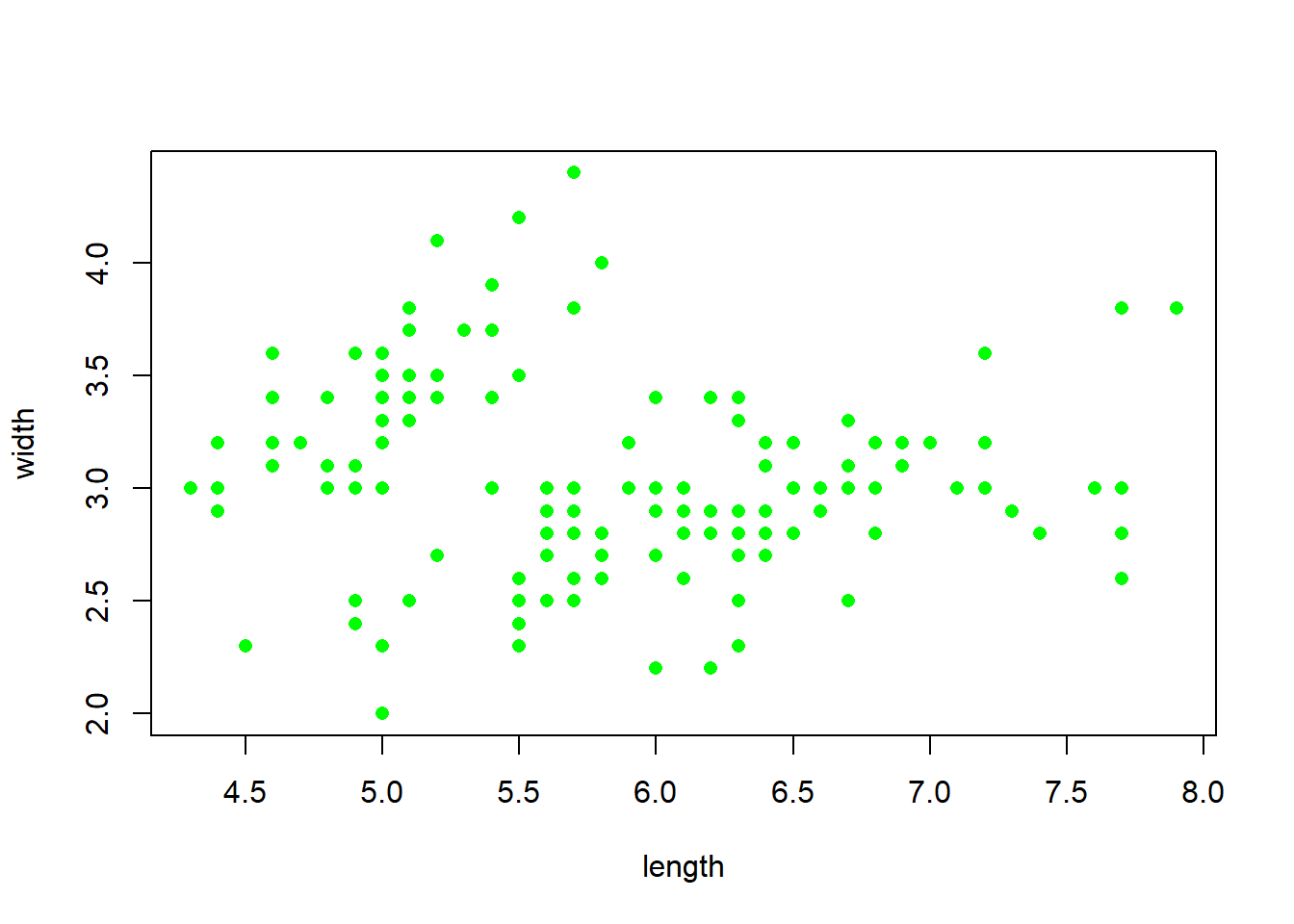

3.1 e

The plot function creates by default a new plot, and using the type argument you can choose the type of plot that you want to plot (default option is “p” which plots points, option “l” plots a line, option “b” plots points connected by a line, and option “n” plots only the plotting window, but no lines or points). On top of an existing plot you can add points or lines via the functions points and lines respectively.

Run the following code to create a data.frame with measurements of grass biomass over time:

grassBiomass <- data.frame(time = 0:50,
                           grass = c(8.4,8.2,5.3,6.7,7.4,12.3,15.0,13.6,9.2,10.5,12.0,
                                     13.6,14.4,11.7,12.0,13.6,12.5,9.3,10.8,12.3,11.3,
                                     14.9,11.2,11.2,5.1,6.4,10.9,11.2,9.8,11.5,9.0,
                                     10.2,6.5,5.0,6.3,6.6,12.5,15.0,12.1,12.0,12.5,
                                     12.0,12.1,13.9,11.3,9.6,11.5,8.2,9.7,10.1,8.5))

Now, create an empty plot window with time on the x-axis and grass on the y-axis (thus use type="n"), and set “Time” and “Grass biomass” to be the axis labels. Then, add a black line to the plot, and after that add solid red points to the plot (both with time on the x-axis and grass on the y-axis).

plot(grassBiomass$time, grassBiomass$grass, type = "n", xlab = "Time", ylab = "Grass biomass")
lines(grassBiomass$time, grassBiomass$grass, col = "black")
points(grassBiomass$time, grassBiomass$grass, col = "red", pch = 16)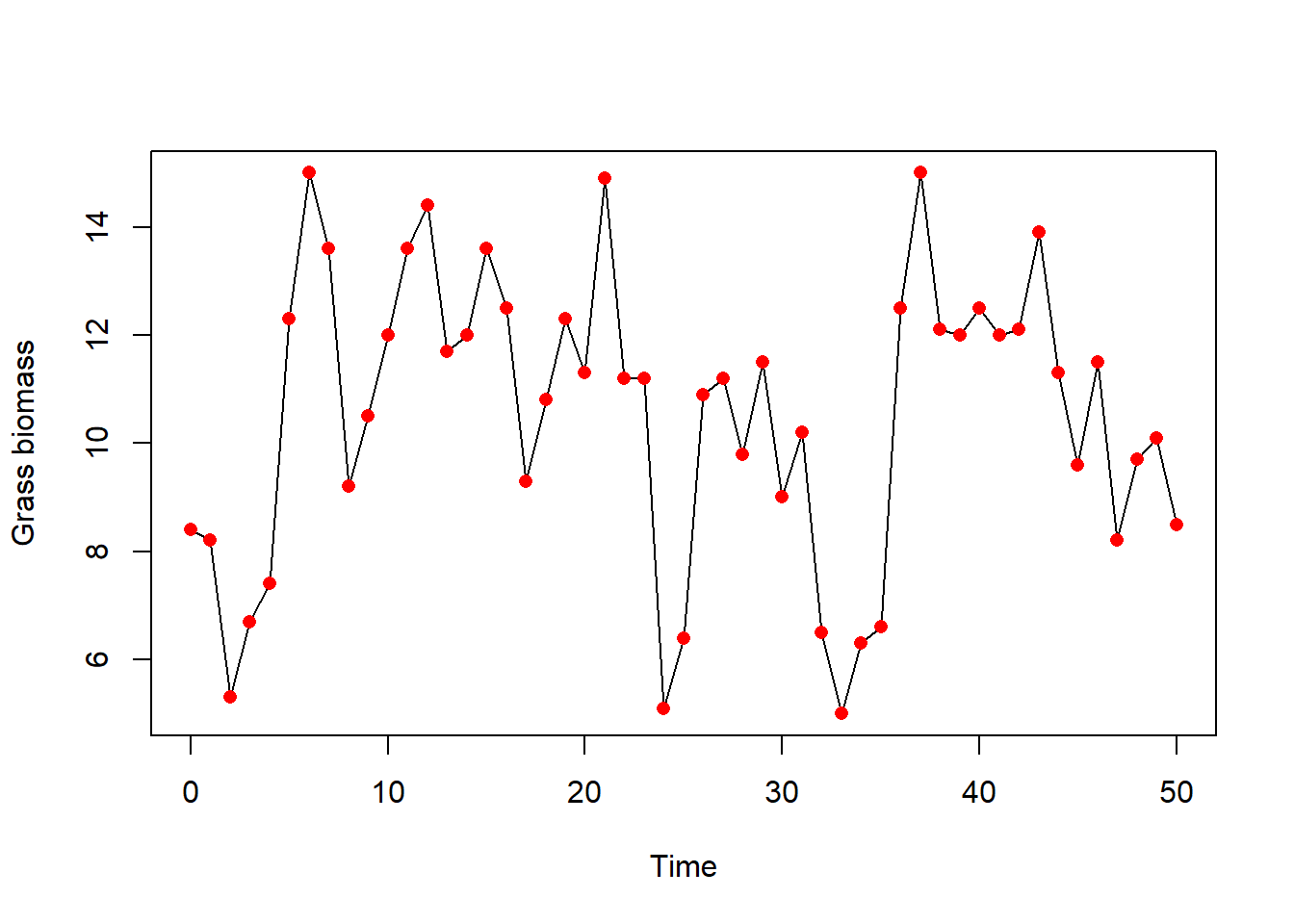

Exercise 3.2

3.2 a

To practice a for-loop: use the iris dataset and print (to the console, using the print function) the value of element on the first row of the first column, the 2^nd row of the 2^nd column, … etc …, up to the 5^th row in the 5^th column.

for(i in 1:5) {
  print(iris[i,i])
}

## [1] 5.1
## [1] 3
## [1] 1.3
## [1] 0.2
## [1] setosa
## Levels: setosa versicolor virginica

3.2 b

Write a new for-loop that prints (to the console) rows 1, 51, and 101. Hint: instead of using e.g. 1:5 as done above, you can use the c() function to create a sequence of values over which the iterator i should iterate.

for(i in c(1,51,101)) {
  print(iris[i,])
}

##   Sepal.Length Sepal.Width Petal.Length Petal.Width Species
## 1          5.1         3.5          1.4         0.2  setosa
##    Sepal.Length Sepal.Width Petal.Length Petal.Width    Species
## 51            7         3.2          4.7         1.4 versicolor
##     Sepal.Length Sepal.Width Petal.Length Petal.Width   Species
## 101          6.3         3.3            6         2.5 virginica

Exercise 3.3

3.3 a

Write your own function with the name myFun that takes 2 function argument as input, call them x and y, and returns an object called z, which is the product of x and the square root of y (using function sqrt).

myFun = function(x, y) {
  z <- x * sqrt(y)
  return(z)
}

3.3 b

Call your function with input value 5 (for x) and 100 (for y): is the output of the function indeed 50?

myFun(x=5, y=100)

## [1] 50

Exercise 3.4

Sometimes, e.g., the coming weeks when analysing models using R, you will not supply a single value as input to a function, but rather a named vector or list with many parameter values and/or state variables. The with function is in such a case a very helpful way to retrieve the elements of a named object in a concise and efficient way.

3.4 a

Retrieve the help-documentation for the with function: what type of object can be passed on to the function as its first argument?

?with
# the first argument (data) may be an environment, a list, a data frame, or an integer

3.4 b

Create a named vector with element names a and b, with values 5 and 3, respectively, and assign it to an object called parms.

parms <- c(a=5, b=3)

3.4 c

Compute the sum of the elements a and b stored in the object parms, using square bracket index notation.

parms[["a"]] + parms[["b"]]

## [1] 8

However, especially with objects containing many different elements, coding in this way can become very tedious. Using the with function, we can access the elements a and b directly using their name (without having to index the elements using parms[["name""]]). The with function can be used with the following syntax:

with(data, expr)

Here, data contains the elements, and expr contains the code that is evaluated. Most conveniently, a list is supplied to the data argument, and the code in expr is bundled within curly brackets {} so that you can even evaluate code that spans many lines.

To convert the object parms into a list, you can use the as.list function:

as.list(parms)

For example, using the parms object created above, you can use the with statement to print the values of elements a and b to the console:

with(as.list(parms),{
  # R statements here, possibly spanning many lines of code
  
  # e.g. print the value of 'a' to the console
  print(a)
  
  # e.g. print the value of 'b' to the console
  print(b)
})

3.4 d

Practice the use of the with function yourself: compute the product of elements a and b without having to index the elements using the square brackets.

with(as.list(parms),{
  a * b
})

## [1] 15

Exercise 3.5

3.5 a

Often, you want to do something multiple times, and store some of its output in a single object. A convenient way to do this is to combine the functionality of a for loop with the flexibility of a list. You can create an empty list using list(), and subsequently assign elements to it using double square bracket notation [[]]. Creates an empty list called myList, and then store each row of the iris dataset as a separate element in the list using a for-loop. Then, check the contents of the object myList by printing the header to the console (function head).

myList <- list()
for(i in 1:nrow(iris)) {
  # store the i-th row of iris as the i-th element in the list
  myList[[i]] <- iris[i,]
}

# check contents
head(myList)

## [[1]]
##   Sepal.Length Sepal.Width Petal.Length Petal.Width Species
## 1          5.1         3.5          1.4         0.2  setosa
## 
## [[2]]
##   Sepal.Length Sepal.Width Petal.Length Petal.Width Species
## 2          4.9           3          1.4         0.2  setosa
## 
## [[3]]
##   Sepal.Length Sepal.Width Petal.Length Petal.Width Species
## 3          4.7         3.2          1.3         0.2  setosa
## 
## [[4]]
##   Sepal.Length Sepal.Width Petal.Length Petal.Width Species
## 4          4.6         3.1          1.5         0.2  setosa
## 
## [[5]]
##   Sepal.Length Sepal.Width Petal.Length Petal.Width Species
## 5            5         3.6          1.4         0.2  setosa
## 
## [[6]]
##   Sepal.Length Sepal.Width Petal.Length Petal.Width Species
## 6          5.4         3.9          1.7         0.4  setosa

Solutions as R script

Download here the code as shown on this page in a separate .r file.