Wageningen University & Research | FEM-31806 | Models for Ecological Systems | FEM | PPS | WEC

This is a code template that you can use as backbone for an R script that implements a model into code in order to solve it numerically, including discontinuous events at discrete points in time.

This template only covers a very basic method to apply discrete events to state variables. See Appendix A and ?events for more information.

Code template

A file containing the code template as shown in the code chunk below can be downloaded here. Places indicated by ... need to be filled out (other parts of the template consist of explanation, and include placeholders for parts that will be completed in later lectures and templates):

# Template 3 - Discrete events
# See: https://wec.wur.nl/mes for explanation and examples

# Load the deSolve library
library(deSolve)

# Define a function that returns a named vector with initial state values
# see Template 1

# Define a function that returns a named vector with parameter values
# see Template 1

# Define a function for the rates of change of the state variables with respect to time
# see Template 1

# Create an events object to specify the discontinuous events at discrete points in time
EventsModelname = list(data = data.frame(var    = ...,  # column name on which the event acts
                                         time   = ... , # timing of the event
                                         value  = ...,  # value of the event
                                         method = ...)) # "replace", "add" or "multiply"

# Numerically solve the model using the ode() function
states <- ode(y = inits,
              times = seq(from = ..., to = ..., by = ...),
              func = RatesModelname,
              parms = ParmsModelname(...),
              method = ...,
              events = EventsModelname)

# Plot
plot(states)

An example with explanation

Let’s continue the model of logistic population growth of population $N$ as developed in Template 1, but now for a population that is subjected to discontinuous events at discrete points in time times. Because in this example we do not have to update any of the functions we need to define: InitLogistic, ParmsLogistic and RatesLogistic, we will use these functions as defined in Template 1 - ODE basics in R.

InitLogistic <- function(N = 5) {
  # Gather function arguments in a named vector
  y <- c(N = N)
  
  # Return the named vector
  return(y)
}

ParmsLogistic <- function(r = 0.3, # intrinsic population growth rate
                          K = 100  # carrying capacity
                          ) {
  # Gather function arguments in a named vector
  y <- c(r = r,
         K = K)
  
  # Return the named vector
  return(y)
}

RatesLogistic <- function(t, y, parms) {
  # use the with() function to be able to access the parameters and states easily
  # remember that the with() function is with(data, expr), where
  # - 'data' is ideally a list with named elements
  #   thus: 'y' and 'parms' are combined using function c and converted using function as.list
  # - 'expr' is an expression (i.e. code) that is evaluated
  #   this can span multiple lines of code when embraced with curly brackets {}
  with(
    as.list(c(y, parms)),{
      
      # Optional: forcing functions: get value of the driving variables at time t (if any)
      # see template 2
      
      # Optional: auxiliary equations

      # Rate equations
      dNdt <- r*N*(1-N/K)
      
      # Gather all rates of change in a vector
      # - the rates should be in the same order as the states (as specified in 'y')
      # - it can be a named vector, but does not need to be
      RATES <- c(dNdt = dNdt)
      
      # Optional: get in/out flow used to compute mass balances (or set MB <- NULL)
      # see template 4
      MB <- NULL

      # Optional: gather auxiliary variables that should be returned (or set AUX <- NULL)
      # - this should be a named vector or list!
      # here we pass the rate of change of N with respect to time back as auxiliary variable
      AUX <- RATES 
      
      # Return result as a list
      # - the first element is a vector with the rates of change (in the same order as 'y')
      # - all other elements are (optional) extra output, which should be named
      outList <- list(c(RATES, # the rates of change of the state variables
                        MB),   # the rates of change of the mass balance terms if MB is not NULL
                      AUX) # optional additional output per time step
      return(outList)
    }
  )
}

Events

Let’s model a population that is subjected to discontinuous events at discrete points in time, where at time 10 $N$ is reduced by 20, at time 20 $N$ is reduced by half, at time 30 $N$ is replaced by the value 25, and at time 40 $N$ is increased by 10.

With deSolve, such discrete events acting on a state can be specified in different ways. Here, we use a easy method that can be used when events occur at known times and when they influence a single state. See Appendix A for another, more versatile, method.

For this simple method, we need to specify a list, with an element called “data”, which is a data.frame that contains information on:

the name of state variable that is affected (column “var”);
the time of the event (column “time”);
the magnitude of the event (column “value”);
event method (column “method”), with options “replace”, “add” and “multiply”.

Let’s create such an object and call this object EventsLogistic:

EventsLogistic = list(data = data.frame(var = c("N", "N", "N", "N"),
                                        time = c(10, 20, 30, 40) ,
                                        value = c(-20, 0.5, 25, 10),
                                        method = c("add", "multiply", "replace", "add")))

Check the created object by printing it to the console:

EventsLogistic

## $data
##   var time value   method
## 1   N   10 -20.0      add
## 2   N   20   0.5 multiply
## 3   N   30  25.0  replace
## 4   N   40  10.0      add

Solving the model

We can now solve the model numerically (requesting output for times from 0 to 50 in time steps of 0.1, using the adaptive stepsize Runge-Kutta integration method “ode45”), while adding the EventsLogistic object to the events function argument:

states <- ode(y = InitLogistic(),
              times = seq(from=0, to=50, by=0.1),
              func = RatesLogistic,
              parms = ParmsLogistic(),
              method = "ode45",
              events = EventsLogistic)

Exploring the solved model

Let’s plot the population’s dynamics, while adding vertical lines and information associated to the discrete events:

plot(states[, "time"], states[, "N"], type = "n", xlab = "Time", ylab = "N") # type="n" for empty plot
abline(v = EventsLogistic$data$time, col = 8, lty = 2) # first add vertical lines
lines(states[, 1], states[, 2]) # then add population dynamics
text(x = EventsLogistic$data$time, y = 10, 
     labels = paste(EventsLogistic$data$method, EventsLogistic$data$value), pos = 4, cex = 0.75)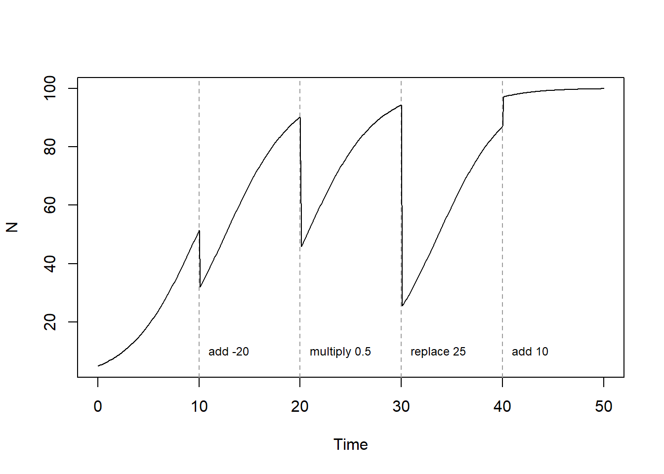

As you can see, it is rather straightforward to include discontinuous events at discrete points in time when solving a model numerically, something that is not possible to do when solving the model (even a simple one) analytically.

Downloadable R script

An R script with the code chunks of the above example can be downloaded here.