Wageningen University & Research | FEM-31806 | Models for Ecological Systems | FEM | PPS | WEC

Aims

Implement the model

Implement the mini-GPLakeR model in R. Use the equations as defined in the mini-model documents. Set up a basic structure to implement the model in R, using the provided R templates. Recall that this means defining (at least) 3 functions that will provide the main input to the deSolve ode function that will be used to numerically solve the model:
- One function that defines the parameter values of the model: call the function “ParmsGPLakeR”, this function will provide input to the ode input argument parms;
- One function that defines the initial values of the state variables (call the function “InitGPLakeR”, this function will provide input to the ode input argument y;
- One function that defines the auxiliary variables and rates equations for all states variables (call the function “RatesGPLakeR”, this function will be the input to the ode input argument func.

Perform technical tests

Run the model for default parameters and initial state values. Check for any programming errors, including possible zero divisions or discontinuities. Ensure to run it for a sufficiently long period of time, e.g. 2000 days, to check if the model reached an equilibrium or resulted in odd behaviour. Run the model using an adaptive stepsize Runge-Kutta integration method: method “ode45”.
Once there are no programming errors, plot the state variables against time: this helps for showing possible left errors. Importantly: does the simulation results reflect the intentions of the model developers?
Vary values of one key parameter. Before doing so, consider the possible effect of this on the state variable – time plots. Make the plots for the default model, but adapted for that single parameter value, and check whether the results follow your expectation. You can repeat this for another key parameter. If the model performs according your expectation, this gives further trust in the model.
Investigate the equilibria in your ecological system by evaluating the state variable – time plots. Does the system come in equilibrium? If not, try longer time periods for the simulation. Does the system ultimately come in equilibrium? If not, why not?
The rate of change of the state variable(s) should not change any longer in equilibrium. Plot therefore the state rates against time. Do these plots correspond with the state – time plots, and show the same results for equilibria?
Do you expect equilibria to differ (reach alternative stable states) when starting with different initial values? If so, vary initial values and check for existence of alternative equilibria.
Check if the computed values for state variables in equilibrium indeed result in rates with a value of 0, as additional check for the implemented formulas. Do this by filling in the computed results in the mathematical equations.
Analyse model behaviour for extreme values of some parameters. Does the model still run correctly, or will there be errors? Is the output what you expect?

Answers

Download here the code as shown on this page in a separate .r file.

Implement the model

See the Templates providing a structure to implement a model in R.

Parameters

The function returning a named vector with parameter values:

ParmsGPLakeR <- function(
    Pload = 2, # Areal P loading (mg P.m-2.d-1)
    z = 2, # Depth (m)
    D = 0.01, # Dilution rate (d-1)
    Rmacr = 0.004, # Macrophyte nutrient retention rate (d-1)
    Rphyt = 0.01, # Phytoplankton nutrient retention rate (d-1)
    Mmacr = 250, # Areal P content of macrophytes at equilibrium during light-limitation (mg P.m-2)
    Mphyt = 250, # Areal P content of phytoplankton at equilibrium during light-limitation (mg P.m-2)
    Gmacr = 0.1, # Maximum per capita growth rate of macrophytes (d-1)
    Gphyt = 0.1, # Maximum per capita growth rate of phytoplankton (d-1)
    Hmacrnutr = 0.01, # Half-saturation constant of nutrient limitation of macrophytes (mg P.m-3)
    Hphytnutr = 0.1, # Half-saturation constant of nutrient limitation of phytoplankton (mg P.m-3)
    Pcrit = 70, # Critical turbidity (mg P.m-2)
    nIntlog = 3, # Parameter in intlog function (-)
    nHill = 30, # Parameter in Hill function (-)
    inocmacr = 0.000001, # Inoculum of macrophytes (mg P.m-2)
    inocphyt = 0.000001, # Inoculum of phytoplankton (mg P.m-2)
    inocratemacr = 0.000001, # Inoculum rate of macrophytes (mg P.m-2.d-1)
    inocratephyt = 0.000001 # Inoculum rate of phytoplankton (mg P.m-2.d-1)
    ) {
  
  # Gather function arguments in a named vector
  y <- c(Pload = Pload,
         z = z,
         D = D,
         Rmacr = Rmacr,
         Rphyt = Rphyt,
         Mmacr = Mmacr,
         Mphyt = Mphyt,
         Gmacr = Gmacr,
         Gphyt = Gphyt,
         Hmacrnutr = Hmacrnutr,
         Hphytnutr = Hphytnutr,
         Pcrit = Pcrit,
         nIntlog = nIntlog,
         nHill = nHill,
         inocmacr = inocmacr,
         inocphyt = inocphyt,
         inocratemacr = inocratemacr,
         inocratephyt = inocratephyt)
  
  # Return
  return(y)
}

Initial conditions

The function returning a named vector with initial values for the 3 state variables:

sPmacr: Areal P content of macrophytes (mg P.m-2);
sPphyt: Areal P content of phytoplankton (mg P.m-2);
sPwater: (Free) P concentration in the water (mg P.m-3):

InitGPLakeR <- function(
    sPmacr = 250, # Areal P content of macrophytes (mg P.m-2)
    sPphyt = 0, # Areal P content of phytoplankton (mg P.m-2)
    sPwater = 0 # (Free) P concentration in the water (mg P.m-3)
    ) {
  
  # Gather initial conditions in a named vector; given names are names for the state variables in the model
  y <- c(sPmacr = sPmacr,
         sPphyt = sPphyt,
         sPwater = sPwater)
  
  # Return
  return(y)
}

Differential equations

The function computing the rates of change of the state variables with respect to time:

RatesGPLakeR <- function(t, y, parms) {
  # use the with() function to be able to access the parameters and states easily
  # remember that the with() function is with(data, expr), where
  # - 'data' is ideally a list with named elements
  #   thus: 'y' and 'parms' are combined using function c and converted using function as.list
  # - 'expr' is an expression (i.e. code) that is evaluated
  #   this can span multiple lines of code when embraced with curly brackets {}
  with(
    as.list(c(y, parms)),{
      
      ### Optional: forcing functions: get value of the driving variables at time t (if any)
      
      ### Optional: auxiliary equations
      Pwater <- max(sPwater, 0)
      LRmacr <- Mmacr * ( 1 - log(exp(nIntlog * (1 - Pload / (Rmacr * Mmacr))) + 1) / log(exp(nIntlog) + 1))
      LRphyt <- Mphyt * (1 - log(exp(nIntlog * (1 - Pload / ((Rphyt + D) * Mphyt))) + 1) / log(exp(nIntlog) + 1))
      State <- Pcrit ^ nHill / (Pcrit ^ nHill + sPphyt ^ nHill)
      Pmacreq <- LRmacr * State
      Pphyteq <- min(max(((Pload - Rmacr * sPmacr) / (Rphyt + D)),0),LRphyt) * State + LRphyt * (1 - State)
      Pwatereq <- ((Pload - (Rphyt + D) * LRphyt) / (z * D)) * (1 - State)
      Macrnutrlim <- Pwater / (Hmacrnutr + Pwater)
      Phytnutrlim <- Pwater / (Hphytnutr + Pwater)
      Hmacrdens <- Rmacr / (Gmacr - Rmacr) # H for density dependence of macrophytes
      Hphytdens <- (Rphyt + D) / (Gphyt - (Rphyt + D)) # H for density dependence of phytoplankton
      Macrdenslim <- Hmacrdens / (Hmacrdens + sPmacr / (Pmacreq + inocmacr))
      Phytdenslim <- Hphytdens / (Hphytdens + sPphyt / (Pphyteq + inocphyt))
      GRmacr <- Gmacr * Macrnutrlim * Macrdenslim
      GRphyt <- Gphyt * Phytnutrlim * Phytdenslim
      
      # Rate equations
      dPmacr <- inocratemacr + GRmacr * sPmacr - Rmacr * sPmacr
      dPphyt <- inocratephyt + GRphyt * sPphyt - (Rphyt + D) * sPphyt
      dPwater <- (Pload - GRmacr * sPmacr - GRphyt * sPphyt) / z - D * Pwater
      
      ### Gather all rates of change in a vector
      # - the rates should be in the same order as the states (as specified in 'y')
      # - it can be a named vector, but does not need to be
      RATES <- c(dPmacr = dPmacr,
                 dPphyt = dPphyt,
                 dPwater = dPwater)
      
      ### Optional: get in/out flow used to compute mass balances (or set MB <- NULL)
      # not included here (thus here use MB <- NULL), see template 3
      MB <- NULL
      
      ### Optional: gather auxiliary variables that should be returned (or set AUX <- NULL)
      # - this should be a named vector or list!
      AUX <- NULL
      
      # Return result as a list
      # - the first element is a vector with the rates of change (in the same order as 'y')
      # - all other elements are (optional) extra output, which should be named
      outList <- list(c(RATES, # the rates of change of the state variables (same order as 'y'!)
                        MB),   # the rates of change of the mass balance terms (or NULL)
                      AUX) # optional additional output per time step
      return(outList)
    })
}

With these 3 functions now defined, the GPLakeR mini-model has been implemented in R code, and the model can now numerically be solved using the ode function from the deSolve package.

Performing technical tests

Use deSolve to integrate the model numerically using the adaptive stepsize Runge-Kutta integration method (“ode45”), here for 2000 days time units in timesteps of 20.

states <- ode(y = InitGPLakeR(),
              times <- seq(from = 0, to = 2000, by = 20),
              parms = ParmsGPLakeR(),
              func = RatesGPLakeR,
              method = "ode45")

Model checks

We split up the testing of the model implementation in two steps: by checking whether the model runs technically and whether the computed results are reasonable.

First, if a model implementation runs technically without errors or important warning messages, it means e.g. that there are no zero divisions and no unexpected discontinuities. We can assess this by plotting state variables versus time or versus each other. If this appears to be correct, we can assess whether the model implementation computes results that are reasonable. First, we can plot the computed results using:

plot(states)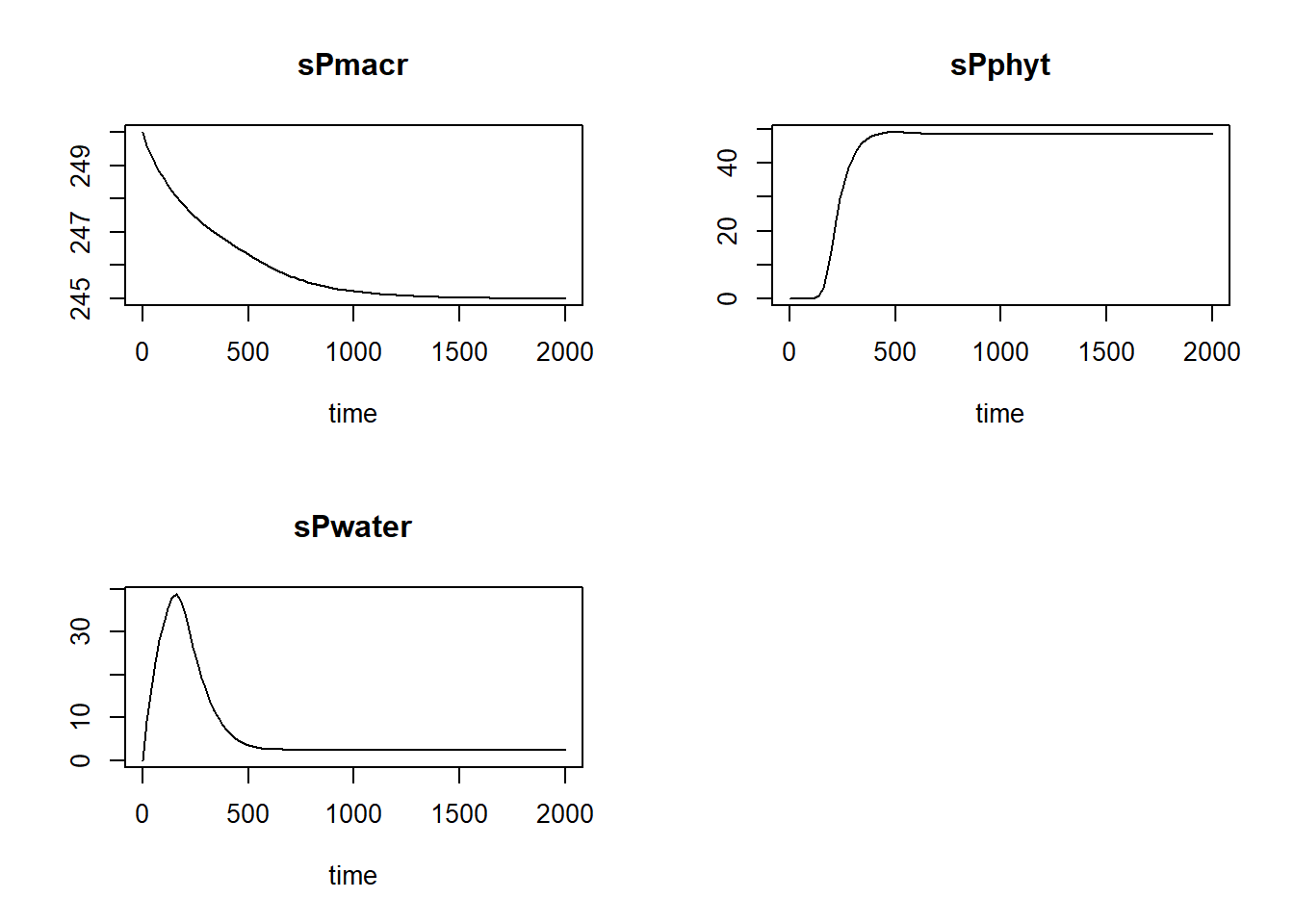

Second, we can check whether the results are reasonable by checking the units of the model implementation, similarly as for the model equations. Of course, if you did everything correctly, the units will be the same, but it is still needed and often programming errors are discovered. The reasonableness of results can also be checked if we know (or expect) that the model (and thus the model application) ought to reach an equilibrium. In that case the (net) rates will become zero. We can discover this by running the model for a long time period with small steps.

Some models will reach an equilibrium state after a period time. Often you have an expectation, if an equilibrium can be expected to occur.

If we want to look at how the rates of change vary over time, and thus not only the values of the state variables, we can do this easily by changing AUX <- NULL into AUX <- RATES in the function defined above that computes the rates of change of the state variables. Then, simply running plot(states) will not only plot the state variables as function of time, but also their rates as function of time.

### SAME as earlier, but with AUX <- RATES
RatesGPLakeR <- function(t, y, parms) {
  # use the with() function to be able to access the parameters and states easily
  # remember that the with() function is with(data, expr), where
  # - 'data' is ideally a list with named elements
  #   thus: 'y' and 'parms' are combined using function c and converted using function as.list
  # - 'expr' is an expression (i.e. code) that is evaluated
  #   this can span multiple lines of code when embraced with curly brackets {}
  with(
    as.list(c(y, parms)),{
      
      ### Optional: forcing functions: get value of the driving variables at time t (if any)
      
      ### Optional: auxiliary equations
      Pwater <- max(sPwater, 0)
      LRmacr <- Mmacr * ( 1 - log(exp(nIntlog * (1 - Pload / (Rmacr * Mmacr))) + 1) / log(exp(nIntlog) + 1))
      LRphyt <- Mphyt * (1 - log(exp(nIntlog * (1 - Pload / ((Rphyt + D) * Mphyt))) + 1) / log(exp(nIntlog) + 1))
      State <- Pcrit ^ nHill / (Pcrit ^ nHill + sPphyt ^ nHill)
      Pmacreq <- LRmacr * State
      Pphyteq <- min(max(((Pload - Rmacr * sPmacr) / (Rphyt + D)),0),LRphyt) * State + LRphyt * (1 - State)
      Pwatereq <- ((Pload - (Rphyt + D) * LRphyt) / (z * D)) * (1 - State)
      Macrnutrlim <- Pwater / (Hmacrnutr + Pwater)
      Phytnutrlim <- Pwater / (Hphytnutr + Pwater)
      Hmacrdens <- Rmacr / (Gmacr - Rmacr) # H for density dependence of macrophytes
      Hphytdens <- (Rphyt + D) / (Gphyt - (Rphyt + D)) # H for density dependence of phytoplankton
      Macrdenslim <- Hmacrdens / (Hmacrdens + sPmacr / (Pmacreq + inocmacr))
      Phytdenslim <- Hphytdens / (Hphytdens + sPphyt / (Pphyteq + inocphyt))
      GRmacr <- Gmacr * Macrnutrlim * Macrdenslim
      GRphyt <- Gphyt * Phytnutrlim * Phytdenslim
      
      # Rate equations
      dPmacr <- inocratemacr + GRmacr * sPmacr - Rmacr * sPmacr
      dPphyt <- inocratephyt + GRphyt * sPphyt - (Rphyt + D) * sPphyt
      dPwater <- (Pload - GRmacr * sPmacr - GRphyt * sPphyt) / z - D * Pwater
      
      ### Gather all rates of change in a vector
      # - the rates should be in the same order as the states (as specified in 'y')
      # - it can be a named vector, but does not need to be
      RATES <- c(dPmacr = dPmacr,
                 dPphyt = dPphyt,
                 dPwater = dPwater)
      
      ### Optional: get in/out flow used to compute mass balances (or set MB <- NULL)
      # not included here (thus here use MB <- NULL), see template 3
      MB <- NULL
      
      ### Optional: gather auxiliary variables that should be returned (or set AUX <- NULL)
      # - this should be a named vector or list!
      AUX <- RATES
      
      # Return result as a list
      # - the first element is a vector with the rates of change (in the same order as 'y')
      # - all other elements are (optional) extra output, which should be named
      outList <- list(c(RATES, # the rates of change of the state variables (same order as 'y'!)
                        MB),   # the rates of change of the mass balance terms (or NULL)
                      AUX) # optional additional output per time step
      return(outList)
    })
}

# solve the model
states <- ode(y = InitGPLakeR(),
              times <- seq(from=0, to=2000, by=20),
              parms = ParmsGPLakeR(),
              func = RatesGPLakeR,
              method = "ode45")

# explore
head(states)

##      time   sPmacr       sPphyt   sPwater      dPmacr       dPphyt   dPwater
## [1,]    0 250.0000 0.000000e+00  0.000000 -0.99999900 1.000000e-06 1.0000000
## [2,]   20 249.5898 4.809886e-05  9.254709 -0.01479456 4.796474e-06 0.4156687
## [3,]   40 249.3107 2.834216e-04 16.786909 -0.01324499 2.350526e-05 0.3401185
## [4,]   60 249.0574 1.438182e-03 22.951159 -0.01211421 1.154142e-04 0.2783596
## [5,]   80 248.8251 7.113070e-03 27.994746 -0.01114380 5.671125e-04 0.2276206
## [6,]  100 248.6110 3.495244e-02 32.110979 -0.01027607 2.776681e-03 0.1850694

plot(states)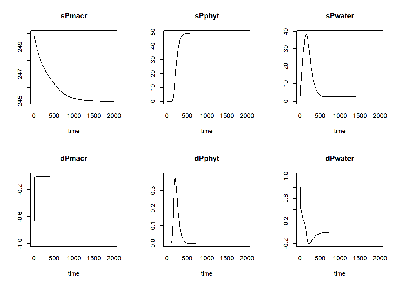

Moreover, we can easily change parameter values or initial state values from their defaults, by including input values to the function calls to functions “ParmsGPLakeR” (input to the argument parms in the ode function call), as well as function “InitGPLakeR” (input to the argument y in the ode function call).

The GPLake-R model can result in alternate stable states, depending on where you start. To demonstrate, let’s solve the model along a gradient in the initial value of P, here a sequence of 101 values from 0 to 5. First, we set a vector with P loading values:

Ploadinit <- seq(from = 0, to = 5, length.out = 101)

Now, we can solve the model for each P loading and store the output in a list (we use a for-loop to solve the model for each value stored in Pload):

outList <- list()
for(i in 1:length(Ploadinit)) {
  outList[[i]] <- ode(y = InitGPLakeR(),
                      times = seq(from = 0, to = 2000, by = 20),
                      parms = ParmsGPLakeR(Pload=Ploadinit[i]),
                      func = RatesGPLakeR,
                      method = "euler")
}

We can simply plot all 100 simulations in 1 set of plots using:

plot(outList[[1]], outList[-1])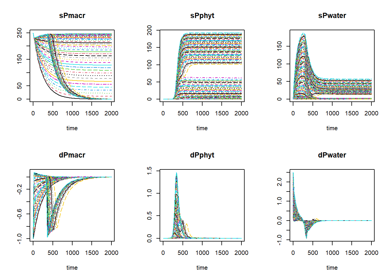

To see how states sPmacr and sPphyt at the end of a simulation depend on the initial value for Pload, we first have to retrieve the values of sPmacr and sPphyt in the last record of the matrices (here we can use the lapply function combined with the unlist to get the last record of a column), and then plot:

sPmacrend <- unlist(lapply(outList, function(x){x[nrow(x),"sPmacr"]}))
sPphytend <- unlist(lapply(outList, function(x){x[nrow(x),"sPphyt"]}))

par(mfrow = c(1,2))
plot(Ploadinit, sPmacrend, type="l", xlab="initial P loading", ylab = "sPmacr")
plot(Ploadinit, sPphytend, type="l", xlab="initial P loading", ylab = "sPphyt")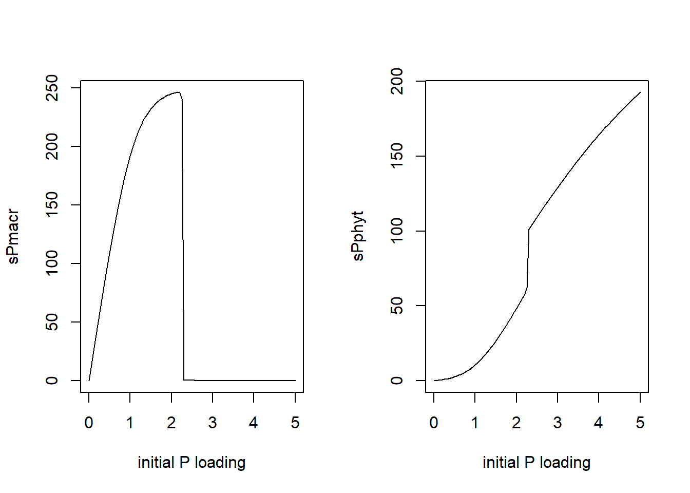

par(mfrow = c(1,1))

What we see is that there is a critical initial P loading that determines in which equilibrium the system will end up.

GPLakeR - Day 2

Aims

Implement the model

Perform technical tests

Answers

Implement the model

Parameters

Initial conditions

Differential equations

Performing technical tests