KISS stands for Keep it Simple Stupid. For modellers this means that models should be made as simple as possible, but not simpler. An adequate model includes only relevant processes that relate to the model objective. A process should only be included in the model if it captures a key component of the system and reduces model error and uncertainty. Detailed processes that seem relevant may not reduce model error (i.e. may not explain much of the observed variation) and only add to model uncertainty. This may be due to a large uncertainty in required process parameter estimates or a limited quantitative understanding of the processes at play. Such processes should be left out or replaced by simpler (e.g. summary) types of process descriptions for which parameters can be measured more easily. For example, a detailed description of photosynthesis in leaves to assess assimilation combined with respiration in various plant organs to estimate net growth rates of a crop is not needed and can better be replaced by a simple growth rate equation based on an easy to measure value for radiation use efficiency.

The analytical solution includes the integration constant and the exact value for every moment in time is known. With this, the change from t=5 to t=10 can be easily computed. Numerical integration is based on step-by-step integration of derivatives which do not include this integration constant. Hence, the states are not known at any point in time but depend on the initial value for these states at a specific moment in time. Therefore, the numerical integration can only start from the moment when all states are known, in this case t=0.

The unit of $C$ is expressed in parts per million (ppm), so $K_c$ must also be in ppm otherwise $C$ and $K_c$ cannot be added. This also means that $P$ is dimensionless (effectively ppm/ppm, a fraction). The units cancel each other out in the ratio.

The maximum value of $P$ is 1. Since $C$ is a concentration, it cannot be smaller than 0. $P$ ranges from 0 (when $C=0$) to (or better close to) a maximum value 1 when $C >> K_c$.

In the previous exercise, we found that the maximum value of $P$ equals 1. At 50% of this maximum, $P$ is thus at 0.5. When the ratio of $C/ (C + K_c)$ is 0.5, the value of $K_c$ equals the value of $C$.

To get $P$ in mg CO₂ m^-2 leaf s^-1, the ratio must be multiplied with a factor (e.g. $Vm$) with the same unit (mg CO₂ m^-2 leaf s^-1). This factor defines the maximum leaf photosynthetic rate (in these units), and the amount of CO₂ absorbed per unit leaf area per second.

distance time ^-1, time^-1, time^-1.

The terms that are added or subtracted should have the same dimensions or units. The dimensions of expressions should be identical at both sides of the equal sign. In multiplication reciprocal dimensions cancel out. In division identical dimensions cancel out. The arguments of exponentials, logarithms and angles should be dimensionless. Note that dimensions refer to length, mass and/or time. When we wish to check the consistency of equations, however, units like meter (or e.g. centimetre), gram (or e.g. kilogram) and hours (or e.g. seconds) must be used. Units thus comprise dimensional analysis, but vice versa this is not true.

1. A sufficient amount of food available should be available for the organisms at all times to support these growth rates;
2. Harmful waste products should be absent or kept at a low level;
3. Abiotic conditions that can affect growth rates, such as temperature, salt concentration and acidity, should be kept constant;
4. Biotic factors that may influence growth rates, such as pests and diseases, should be absent or be kept at a constant level.

The slopes represent the time derivatives (dy/dt) of the variable on the y-axis.

The dimension is change of state/t or (the dimension of the state variable) • time-1.

The numerical value of the slope in the Figure 1.5d does not change; it is equal to the constant $c$. The numerical values of the slopes in the Figure 1.5e and 1.5f increase and decrease with time, respectively.

The graphs give the slope as a function of time. These time derivatives are constant, increasing and decreasing with time, respectively.

The results of the different calculations:

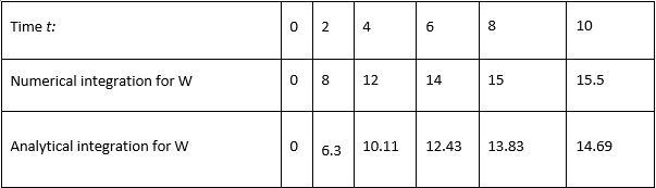
You can download an Excel spreadsheet with the calculations here.

The resulting plot:

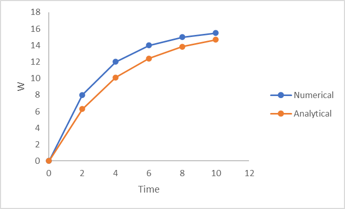
The numerical solution (in blue) overestimates the value of the state variable compared to the analytical solution (in red). This is because the numerical approach assumes that the rate is constant during the time interval of integration, while the rate is in fact decreasing continuously.

When the maximum water level is reached. This is the case after a long time, in principle when $t$ approaches infinity.

The process is twice as slow.

For $\Delta t = 1 · c^{-1} = \tau$, the tank is filled after one time step; no inflow occurs thereafter.

For $\Delta t = 1.5 · c^{-1} = 1.5 · \tau$, the amount of water in the tank oscillates around the equilibrium level, but eventually settles at this level.

For $\Delta t = 2 · c^{-1} = 2 · \tau$, an oscillation around the equilibrium level between the limits 0 and 2 × $W_m$ is obtained.

For $\Delta t = 2.5 · c^{-1} = 2.5 · \tau$, the result is an oscillation with divergence.

No answer given, but oscillations can be observed.

For a ratio $\Delta t / c^{-1} = \Delta t / \tau ≥ 1$ the results do not reflect reality at all.

Taking into account the calculations in Exercise 1.4, the ratio $\Delta t / \tau$ should be smaller than 0.5. As a rule of thumb, and a safe upper limit for the choice of $\Delta t$, $\Delta t$ should be smaller or equal to $0.1 × \tau$.

The time coefficients can be calculated by dividing the time interval by the rate of change ($\Delta t / c^{-1}$). Hence, the time coefficients are: 0.67, 5 and 20 year.

One tenth of $\tau$. However, these data should be rounded off to the nearest smaller value that is an integral fraction of the output interval. For instance, 0.067 will become 0.05, but 0.5 and 2 years may be appropriate for output intervals.

Analytical 271.83 after 5 years. Numerical: 259.37 after 5 years.

No answer given.

During $\Delta t$ the rate of increase is assumed to be constant, but in fact it increases exponentially, as is shown in the graph. After the first time interval the amount is thus underestimated, and consequently the rate for the next time interval is underestimated, and so on. As time proceeds the discrepancy between the numerical and analytical solution becomes larger. This error propagation will be discussed in Chapter 6.

In a positive feedback loop like exponential growth, the change is directed away from the equilibrium state, so the extrapolation of the tangent must be reversed, and directed towards the unstable equilibrium state; the tangent cuts the horizontal equilibrium line (the x-axis), where the value of the state variable equals zero, one time coefficient interval earlier: