Logistic growth

Let’s use the example of logistic growth as defined in Template 1:

# Define a function that returns a named vector with initial state values
InitLogistic <- function(N = 5) {
  # Gather function arguments in a named vector
  y <- c(N = N)
  
  # Return the named vector
  return(y)
}

# Define a function that returns a named vector with parameter values
ParmsLogistic <- function(r = 0.3, # intrinsic population growth rate
                          K = 100 # carrying capacity
                          ){
  # Gather function arguments in a named vector
  y <- c(r = r,
         K = K)
  
  # Return the named vector
  return(y)
}

# Define a function for the rates of change of the state variables with respect to time
RatesLogistic <- function(t, y, parms) {
  # use the with() function to be able to access the parameters and states easily
  # remember that the with() function is with(data, expr), where
  # - 'data' is ideally a list with named elements
  #   thus: 'y' and 'parms' are combined using function c and converted using function as.list
  # - 'expr' is an expression (i.e. code) that is evaluated
  #   this can span multiple lines of code when embraced with curly brackets {}
  with(
    as.list(c(y, parms)),{
      
      # Optional: forcing functions: get value of the driving variables at time t (if any)
      # see template 2
      
      # Optional: auxiliary equations

      # Rate equations
      dNdt <- r*N*(1-N/K)
      
      # Gather all rates of change in a vector
      # - the rates should be in the same order as the states (as specified in 'y')
      # - it can be a named vector, but does not need to be
      RATES <- c(dNdt = dNdt)
      
      # Optional: get in/out flow used to compute mass balances (or set MB <- NULL)
      # see template 4
      MB <- NULL

      # Optional: gather auxiliary variables that should be returned (or set AUX <- NULL)
      # - this should be a named vector or list!
      # here we pass the rate of change of N with respect to time back as auxiliary variable
      AUX <- RATES 
      
      # Return result as a list
      # - the first element is a vector with the rates of change (in the same order as 'y')
      # - all other elements are (optional) extra output, which should be named
      outList <- list(c(RATES, # the rates of change of the state variables
                        MB),   # the rates of change of the mass balance terms if MB is not NULL
                      AUX) # optional additional output per time step
      return(outList)
    }
  )
}

After having defined these functions, we can solve the model using the ode function and plot the results:

states <- ode(y = InitLogistic(),
              times = seq(from = 0, to = 100, by = 0.1),
              func = RatesLogistic,
              parms = ParmsLogistic(),
              method = "ode45")
plot(states)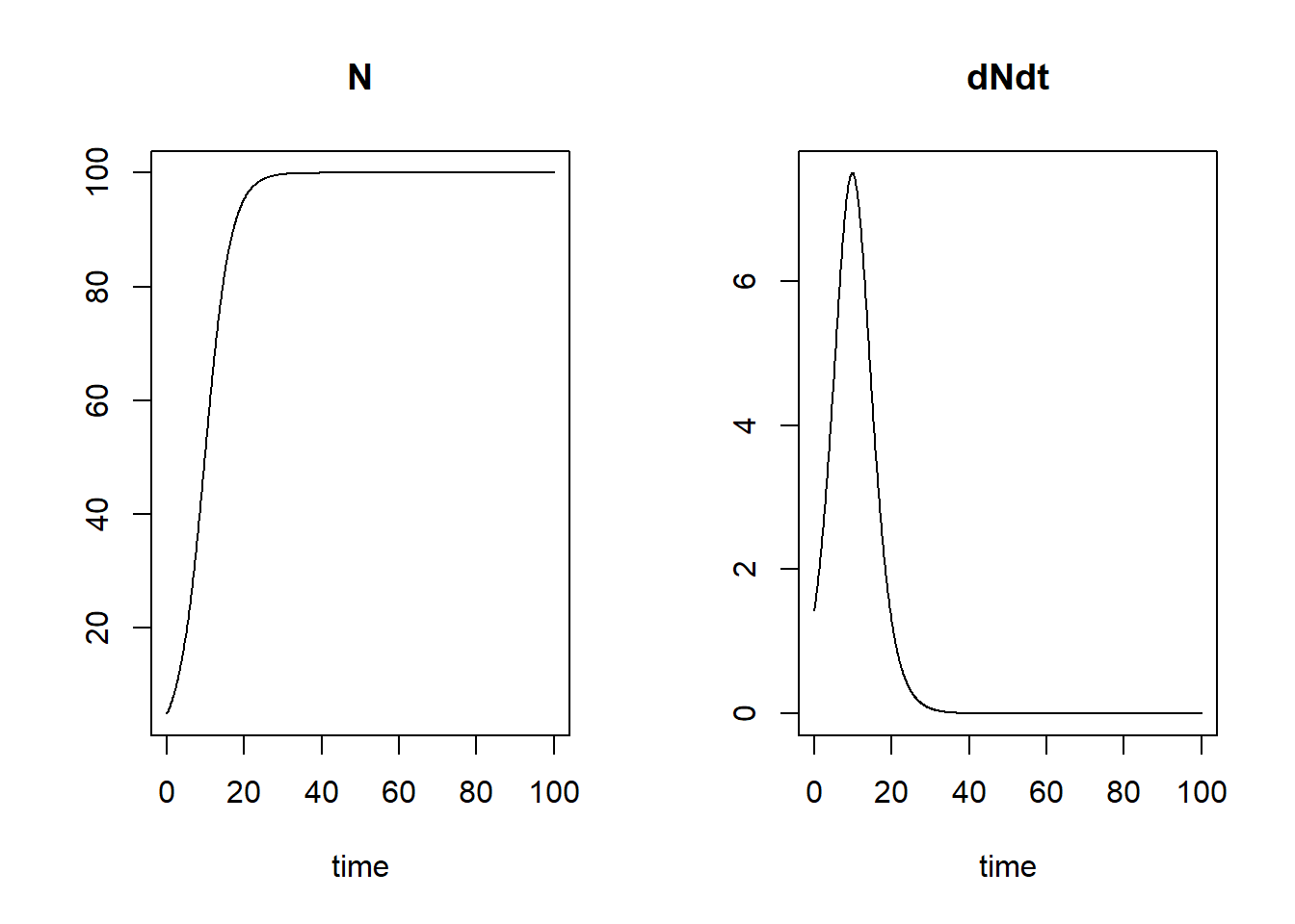

Triggering early termination

If we provide a root function but not an event function, than the simulation will stop at a root. Therefore, let’s create a root function, called root, that triggers a root when the population size $N$ reaches 99% of the carrying capacity $K$ (i.e. a root is triggered when this function returns the value 0):

# Root function when N == 0.99*K
root <- function(t, y, parms) {
  # we use the with() function in a similar way to its use in the RatesLogistic function
  # so that we can easily refer to parameters and state variables by their name(s)
  with(
    as.list(c(t=t, y, parms)),{
      r <- N - (0.99*K) # difference between N and 99% of K: thus: value 0 when N equals 99% of K
      return(r) # then r == 0 this triggers a root
    })
}

After defining this root function, we can simulate the population and stop the simulation when we supply the root function but do not supply an event function. Thus, we pass object root as input to argument rootfunc, yet the events argument still needs input: as earlier this needs to be a list, but now with values of elements “func” and “root”:

• in element “func” we need to specify the event function; here we do not supply the event function because our intent is early termination of the simulation, therefore we assign it the value NULL;
• in element “root” we need to indicate (with a logical, value, thus either TRUE or FALSE) whether we supply a root function to input argument rootfunc. Here we set it to TRUE since be are supplying a root function. However, we may not always need to supply a root function, as we can also supply an event function along with specified “time” values during which the event function will be called.

Apart from supplying the events list and root function, we set the integration method to “lsoda”, as the “ode45” method used in the templates can not handle root functions:

states <- ode(y = InitLogistic(),
              times = seq(from = 0, to = 100, by = 0.1),
              func = RatesLogistic,
              parms = ParmsLogistic(),
              method = "lsoda", # "ode45" does not handle root functions, but "lsoda" does
              events = list(func = NULL,  # NULL: therefore the simulation is stopped at a root
                            root = TRUE), # specifying that there is a root function
              rootfunc = root)            # the defined root function
plot(states)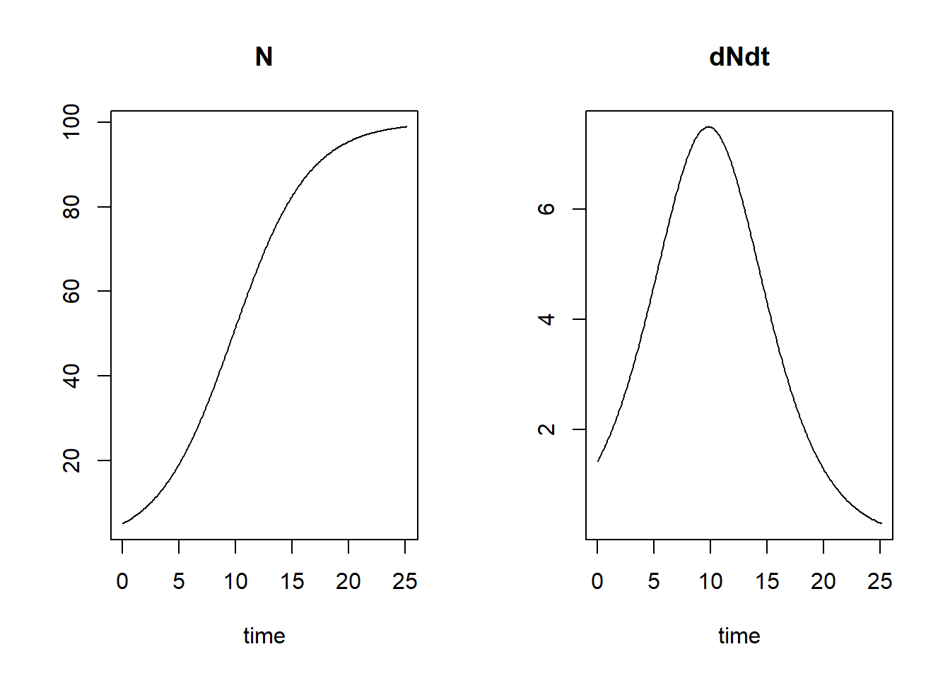

We see that the population reaches 99% of its carrying capacity around time 25, therefore the simulation is stopped and not continued till time 100.

Events at specified times

So demonstrate how we can use an event function that acts on state variables at pre-defined times, let’s simulate the population $N$ for 50 time units, and remove 25% of the population at times 10, 20, 30 and 40. For this, we need to specify an event function that removes 25% of the state variable at the specified times (thus, we replace $N$ by $0.75*N$), and we need to specify the times at which this event function is applied:

# specify event function
eventfun <- function(t, y, parms) {
  y["N"] <- 0.75 * y["N"]
  return(y)
}

# solve the model
states <- ode(y = InitLogistic(),
              times = seq(from = 0, to = 50, by = 0.1),
              func = RatesLogistic,
              parms = ParmsLogistic(),
              method = "ode45",
              events = list(func = eventfun, # the event function, called at times in "time"
                            time = c(10,20,30,40), # the time at which the event function is applied
                            root = FALSE)) # this specifies that we do not supply a root function
                                           # thus: the event function is called at the specified times

# plot the simulation
plot(states)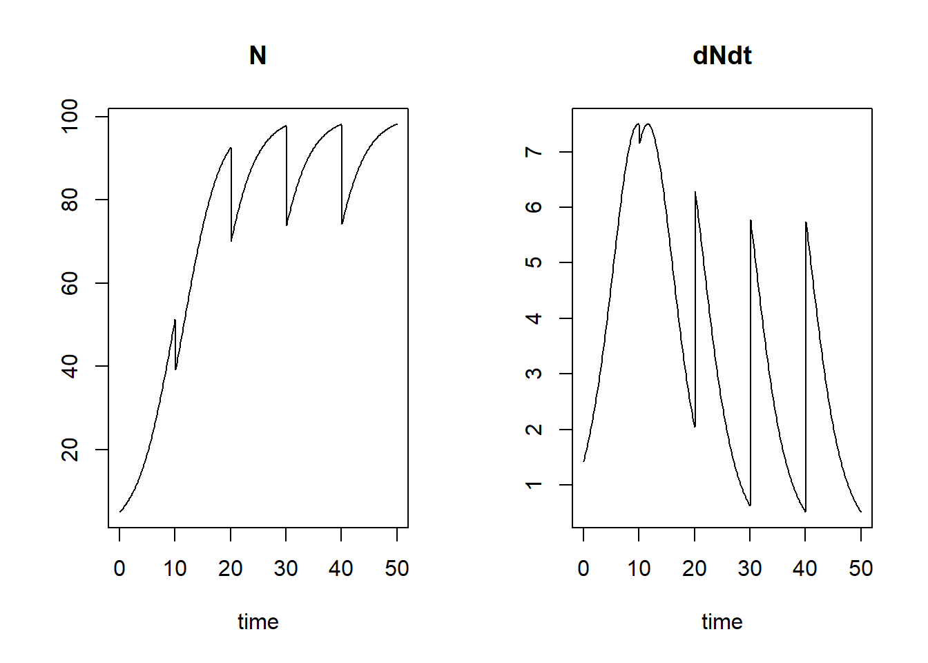

Events triggered by a root

By supplying both an event function as well as a root function, we can apply events to a state variables when some condition is met. For example, we can reduce a population by 25% when the population is large enough, e.g. when the population is at 99% of its carrying capacity $K$:

# root function when N == 0.99*K
root <- function(t, y, parms) {
  # we use the with() function in a similar way to its use in the RatesLogistic function
  # so that we can easily refer to parameters and state variables by their name(s)
  with(
    as.list(c(t=t, y, parms)), {
      r <- N - (0.99*K) # difference between N and 99% of K: thus: value 0 when N equals 99% of K
      return(r) # then r == 0 this triggers a root
    })
}

# specify event function
eventfun <- function(t, y, parms) {
  y["N"] <- 0.75 * y["N"]
  return(y)
}

# solve the model
states <- ode(y = InitLogistic(),
              times = seq(from = 0, to = 50, by = 0.1),
              func = RatesLogistic,
              parms = ParmsLogistic(),
              method = "lsoda",
              events = list(func = eventfun, # the event function, called at times in "time"
                            root = TRUE),    # this specifies that we do supply a root function
              rootfunc = root)

# plot the simulation
plot(states)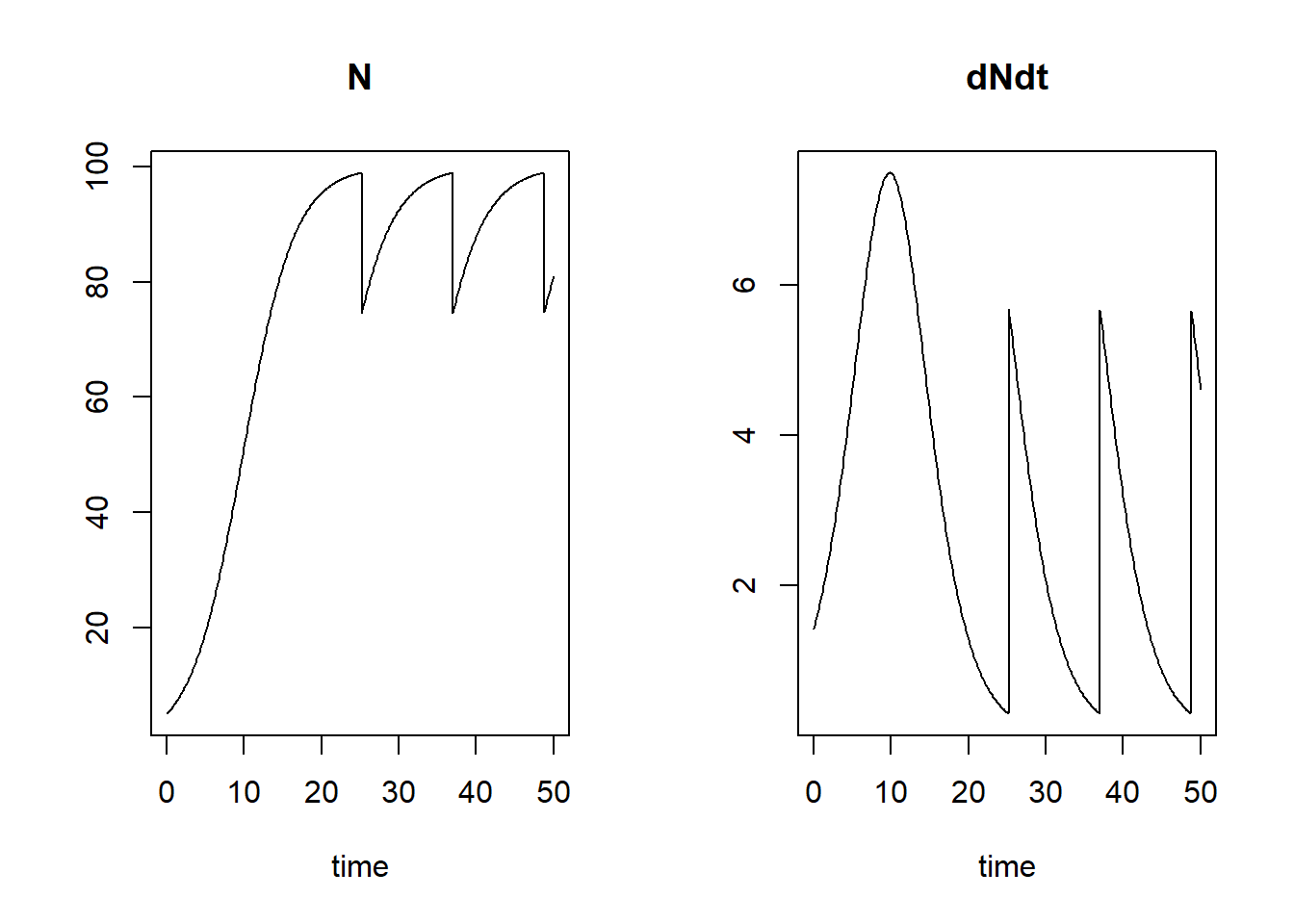

Mass balances and events

This topic is dealt with in Appendix B.

Downloadable R script

An R script with the code chunks of the above example can be downloaded here.