Compare integration methods

To check for the difference between Euler and Runge-Kutta integration, let’s solve the model numerically for 2000 time-units in time-steps of 1, 5 and 10 (the fixed time-step of the euler method), as well as with a variable time-step Runge-Kutta method (ode45, here with output every time-step):

states_rk <- ode(y = InitGPLakeR(sPmacr = 250,
                                sPphyt = 0,
                                sPwater = 0),
                 times = seq(from = 0, to = 2000, by = 1),
                 parms = ParmsGPLakeR(),
                 func = RatesGPLakeR,
                 method = "ode45")

delt <- 1
states_euler1 <- ode(y = InitGPLakeR(sPmacr = 250,
                                sPphyt = 0,
                                sPwater = 0),
                 times = seq(from = 0, to = 2000, by = delt),
                 parms = ParmsGPLakeR(),
                 func = RatesGPLakeR,
                 method = "euler")

delt <- 5
states_euler2 <- ode(y = InitGPLakeR(sPmacr = 250,
                                sPphyt = 0,
                                sPwater = 0),
                 times = seq(from = 0, to = 2000, by = delt),
                 parms = ParmsGPLakeR(),
                 func = RatesGPLakeR,
                 method = "euler")

delt <- 10
states_euler3 <- ode(y = InitGPLakeR(sPmacr = 250,
                                sPphyt = 0,
                                sPwater = 0),
                 times = seq(from = 0, to = 2000, by = delt),
                 parms = ParmsGPLakeR(),
                 func = RatesGPLakeR,
                 method = "euler")

We can have a look at the output of the last time-steps (for all 4 solutions):

tail(states_rk)

##         time   sPmacr   sPphyt  sPwater        dPmacr       dPphyt       dPwater
## [1996,] 1995 244.9865 48.52819 2.475831 -2.169418e-05 2.335407e-06 -2.428463e-06
## [1997,] 1996 244.9864 48.52819 2.475829 -2.161492e-05 2.326873e-06 -2.419587e-06
## [1998,] 1997 244.9864 48.52819 2.475827 -2.153595e-05 2.318370e-06 -2.410743e-06
## [1999,] 1998 244.9864 48.52819 2.475824 -2.145727e-05 2.309899e-06 -2.401932e-06
## [2000,] 1999 244.9864 48.52820 2.475822 -2.137888e-05 2.301458e-06 -2.393153e-06
## [2001,] 2000 244.9864 48.52820 2.475819 -2.130078e-05 2.293049e-06 -2.384406e-06

tail(states_euler1)

##         time   sPmacr   sPphyt  sPwater        dPmacr       dPphyt       dPwater
## [1996,] 1995 244.9859 48.52825 2.475770 -1.967020e-05 2.117487e-06 -2.201801e-06
## [1997,] 1996 244.9859 48.52825 2.475767 -1.959821e-05 2.109735e-06 -2.193738e-06
## [1998,] 1997 244.9859 48.52825 2.475765 -1.952648e-05 2.102012e-06 -2.185706e-06
## [1999,] 1998 244.9858 48.52825 2.475763 -1.945501e-05 2.094317e-06 -2.177703e-06
## [2000,] 1999 244.9858 48.52826 2.475761 -1.938380e-05 2.086651e-06 -2.169729e-06
## [2001,] 2000 244.9858 48.52826 2.475759 -1.931286e-05 2.079012e-06 -2.161784e-06

tail(states_euler2)

##        time   sPmacr   sPphyt  sPwater        dPmacr       dPphyt       dPwater
## [396,] 1975 244.9839 48.52846 2.475543 -1.226647e-05 1.320395e-06 -1.372837e-06
## [397,] 1980 244.9838 48.52847 2.475536 -1.204199e-05 1.296229e-06 -1.347708e-06
## [398,] 1985 244.9838 48.52848 2.475530 -1.182161e-05 1.272505e-06 -1.323038e-06
## [399,] 1990 244.9837 48.52848 2.475523 -1.160527e-05 1.249216e-06 -1.298820e-06
## [400,] 1995 244.9836 48.52849 2.475516 -1.139289e-05 1.226352e-06 -1.275046e-06
## [401,] 2000 244.9836 48.52850 2.475510 -1.118440e-05 1.203908e-06 -1.251706e-06

tail(states_euler3)

##        time   sPmacr   sPphyt  sPwater        dPmacr       dPphyt       dPwater
## [196,] 1950 244.9811 48.52876 2.475237 -2.241715e-06 2.412833e-07 -2.508351e-07
## [197,] 1960 244.9811 48.52876 2.475234 -2.159667e-06 2.324521e-07 -2.416540e-07
## [198,] 1970 244.9811 48.52876 2.475232 -2.080622e-06 2.239441e-07 -2.328090e-07
## [199,] 1980 244.9811 48.52877 2.475229 -2.004470e-06 2.157475e-07 -2.242877e-07
## [200,] 1990 244.9811 48.52877 2.475227 -1.931106e-06 2.078509e-07 -2.160783e-07
## [201,] 2000 244.9810 48.52877 2.475225 -1.860426e-06 2.002433e-07 -2.081694e-07

Now, you can plot all solutions together in a single figure using:

plot(states_rk, states_euler1,states_euler2, states_euler3)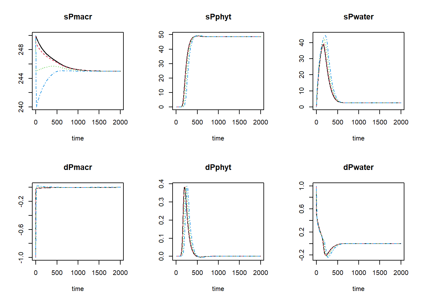

The black line now is the Runge-Kutta solution (with variable time-step), the dashed red line is the first Euler solution (with time-step of 1), the dashed green line is the second Euler solution (with time-step of 5), and the dashed blue line is the third Euler solution (with time-step of 10). To focus a bit more on the first time steps, we can limit the x-axis to a range between 0 and 400 using the xlim argument:

plot(states_rk, states_euler1,states_euler2, states_euler3, xlim=c(0,400))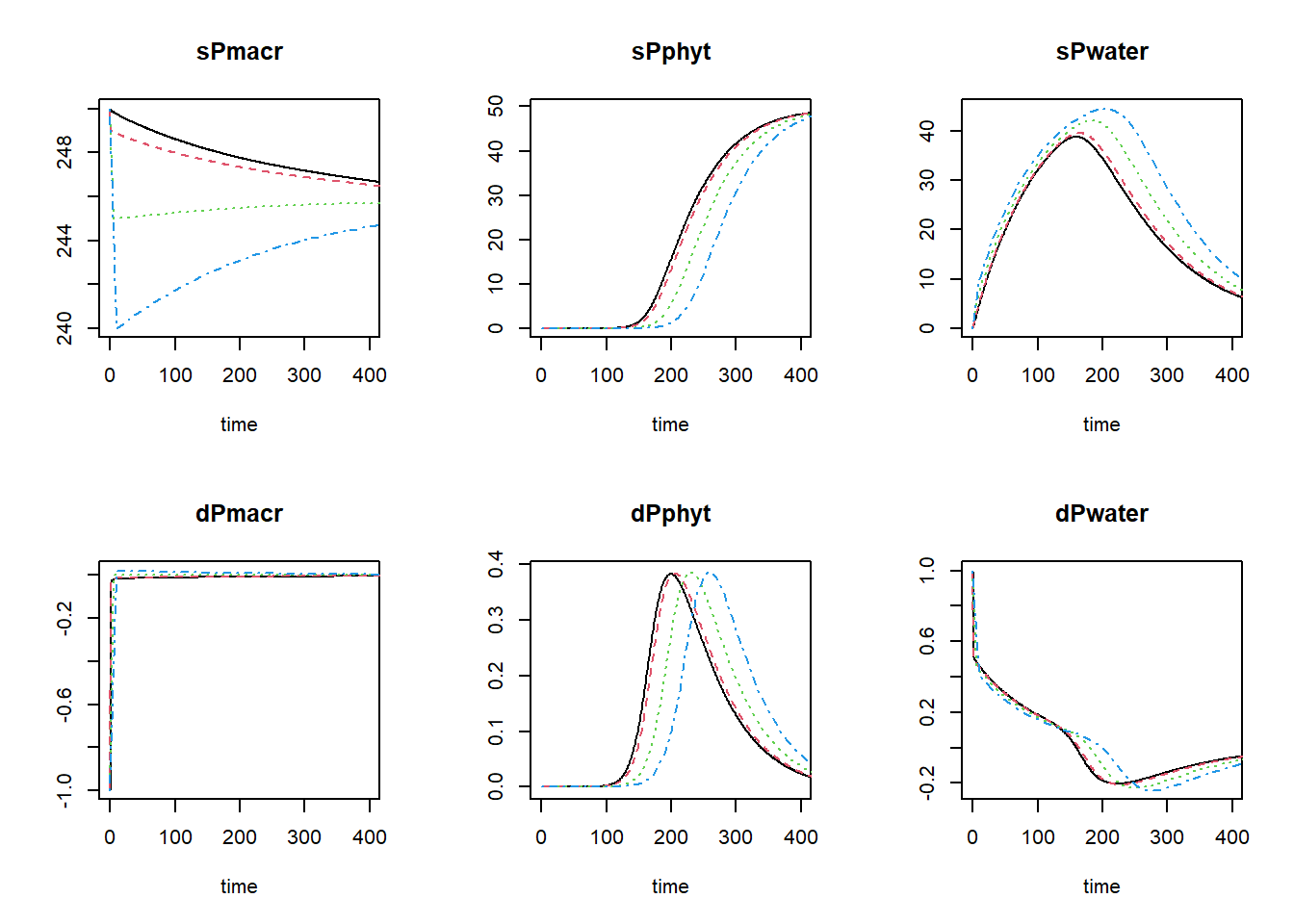

We see that for sPmacr, sPphyt and sPwater the solution with Euler integration at a larger time-step is quite some difference from the Runge-Kutta solution or the Euler solution with a small time-step!

To get the relative difference between the integration methods at time 2000 (here as a fraction of the reference ode45, rounded off to 4 digits):

round(100 * tail(states_euler1, 1)[,-1] / tail(states_rk,1)[,-1], 4)

##   sPmacr   sPphyt  sPwater   dPmacr   dPphyt  dPwater 
##  99.9998 100.0001  99.9975  90.6674  90.6659  90.6634

round(100 * tail(states_euler2, 1)[,-1] / tail(states_rk,1)[,-1], 4)

##   sPmacr   sPphyt  sPwater   dPmacr   dPphyt  dPwater 
##  99.9989 100.0006  99.9875  52.5070  52.5025  52.4955

round(100 * tail(states_euler3, 1)[,-1] / tail(states_rk,1)[,-1], 4)

##   sPmacr   sPphyt  sPwater   dPmacr   dPphyt  dPwater 
##  99.9978 100.0012  99.9760   8.7341   8.7326   8.7305

and here as a relative difference:

round(100 * abs ( (tail(states_euler1, 1)[,-1] - tail(states_rk,1)[,-1]) / tail(states_rk,1)[,-1] ), 4)

##  sPmacr  sPphyt sPwater  dPmacr  dPphyt dPwater 
##  0.0002  0.0001  0.0025  9.3326  9.3341  9.3366

round(100 * abs ( (tail(states_euler2, 1)[,-1] - tail(states_rk,1)[,-1]) / tail(states_rk,1)[,-1] ), 4)

##  sPmacr  sPphyt sPwater  dPmacr  dPphyt dPwater 
##  0.0011  0.0006  0.0125 47.4930 47.4975 47.5045

round(100 * abs ( (tail(states_euler3, 1)[,-1] - tail(states_rk,1)[,-1]) / tail(states_rk,1)[,-1] ), 4)

##  sPmacr  sPphyt sPwater  dPmacr  dPphyt dPwater 
##  0.0022  0.0012  0.0240 91.2659 91.2674 91.2695

These values indicate that after long time (2000 time units), there is not much difference between the integration methods and time-steps, as the system has approached the equilibrium. However, as can be seen in the figures above the Euler integration method with smaller time-step better approaches the variable time-step Runge-Kutta method. Using the Euler integration method, when the time-step increases, the deviation from the Runge-Kutta solution increases. Thus, this pattern demonstrates the expected pattern of time-step convergence.

Therefore, if we compute the relative difference between the Euler solutions and the Runge-Kutta solution at time 400, the solution with a time-step of 1 still is within 1% of the Runge-Kutta solution (for sPmacr and sPphyt), but the other time steps are close to or above 1%:

doTime <- 400
round(100 * abs(subset(states_euler1, time == doTime) - subset(states_rk, time == doTime)) / 
        subset(states_rk, time == doTime), 4)

##   sPmacr   sPphyt  sPwater   dPmacr   dPphyt  dPwater 
##   0.0781   0.1426   4.9974 -19.6293   9.6375  -7.1269

round(100 * abs(subset(states_euler2, time == doTime) - subset(states_rk, time == doTime)) / 
        subset(states_rk, time == doTime), 4)

##    sPmacr    sPphyt   sPwater    dPmacr    dPphyt   dPwater 
##    0.4163    0.9759   27.6739 -103.3690   55.9459  -38.3758

round(100 * abs(subset(states_euler3, time == doTime) - subset(states_rk, time == doTime)) / 
        subset(states_rk, time == doTime), 4)

##    sPmacr    sPphyt   sPwater    dPmacr    dPphyt   dPwater 
##    0.8484    2.8542   63.4037 -208.8010  137.4064  -84.5211

To get the information needed to compute the time coefficients (the value of the state variables when the system is in equilibrium, but also the rates of change of the state variables over time), we have to change AUX <- NULL in function RatesGPLakeR to AUX <- RATES.

##      time   sPmacr       sPphyt   sPwater      dPmacr       dPphyt   dPwater
## [1,]    0 250.0000 0.000000e+00  0.000000 -0.99999900 1.000000e-06 1.0000000
## [2,]   20 249.5898 4.809886e-05  9.254709 -0.01479456 4.796474e-06 0.4156687
## [3,]   40 249.3107 2.834216e-04 16.786909 -0.01324499 2.350526e-05 0.3401185
## [4,]   60 249.0574 1.438182e-03 22.951159 -0.01211421 1.154142e-04 0.2783596
## [5,]   80 248.8251 7.113070e-03 27.994746 -0.01114380 5.671125e-04 0.2276206
## [6,]  100 248.6110 3.495244e-02 32.110979 -0.01027607 2.776681e-03 0.1850694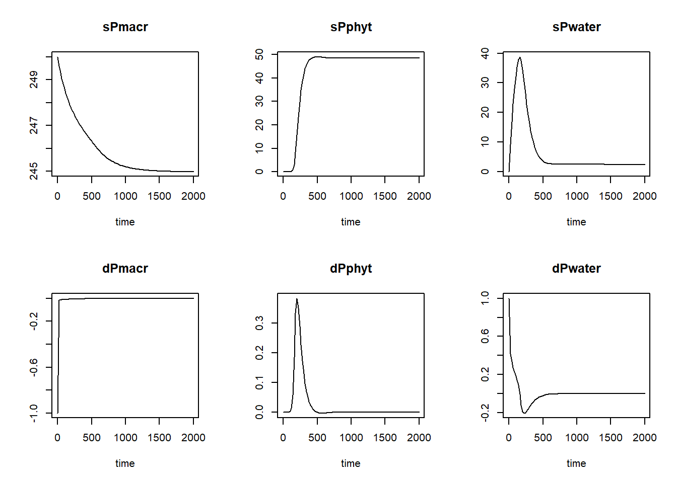

Then, we can define a function that computes the time coefficient; it needs as input a solved model, as well as the time at which the system has reached equilibrium. With this information, we can compute the time coefficients:

tcGPLakeR <- function(states, time_equil) {
  # Find index for row with states that are in equilibrium
  ii <- which(states[,"time"] == time_equil)
  
  # Compute TC for all states using general TC formula
  TC <- data.frame(time = states[,"time"],
                   TC_sPmacr = abs( (states[,"sPmacr"] - states[ii,"sPmacr"]) / states[,"dPmacr"] ),
                   TC_sPphyt = abs( (states[,"sPphyt"] - states[ii,"sPphyt"]) / states[,"dPphyt"] ),
                   TC_sPwater = abs( (states[,"sPwater"] - states[ii,"sPwater"]) / states[,"dPwater"] ))
  return(TC)
}

With a solved model, we can now thus compute the time coefficients, and plot how they vary over time:

states_rk <- ode(y = InitGPLakeR(sPmacr = 250,
                                sPphyt = 0,
                                sPwater = 0),
                 times = seq(from = 1, to = 2000, by = 1),
                 parms = ParmsGPLakeR(),
                 func = RatesGPLakeR,
                 method = "ode45")

TC <- tcGPLakeR(states=states_rk, time_equil = 2000)

par(mfrow = c(2,3)) # reset using par(mfrow = c(1,1)) after plotting the plots

plot(states_rk[,"time"], states_rk[,"sPmacr"], ylab="sPmacr", xlab="time", type="l", col = "black")
plot(states_rk[,"time"], states_rk[,"sPphyt"], ylab="sPphyt", xlab="time", type="l", col = "black")
plot(states_rk[,"time"], states_rk[,"sPwater"], ylab="sPwater", xlab="time", type="l", col = "black")

plot(TC[,"time"], TC[,"TC_sPmacr"], ylab="TC sPmacr", xlab="time", type="l", col = "black")
plot(TC[,"time"], TC[,"TC_sPphyt"], ylab="TC sPphyt", xlab="time", type="l", col = "black")
plot(TC[,"time"], TC[,"TC_sPwater"], ylab="TC sPwater", xlab="time", type="l", col = "black")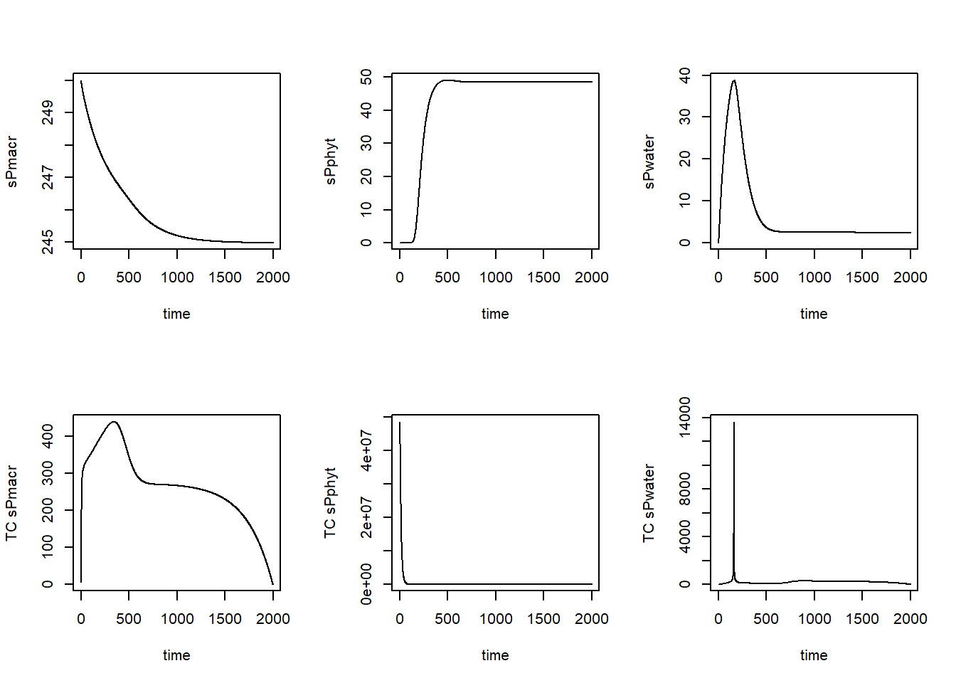

As we can see, the time coefficients vary quite a bit over time. We may be interested in the minimum time coefficient during times where the system is not yet in equilibrium. Let’s say from the plots that this is up to time 800. We can thus compute the minimum time coefficient up to that time:

TC_sub = subset(TC, time <= 800)
min(TC_sub$TC_sPmacr)

## [1] 5.013633

min(TC_sub$TC_sPphyt)

## [1] 0.03182582

min(TC_sub$TC_sPwater)

## [1] 0.09464382

Thus, the minimum time coefficient seems to be ca. 0.032.

Mass balances tests

To analyse the mass balance of the model, let’s copy-paste the “InitGPLakeR” and “RatesGPLakeR” functions as defined earlier, and add 6 extra states (in and out per state variable sPmacr, sPphyt, and sPwater), at initial value 0:

InitGPLakeR <- function(sPmacr = 250, # Areal P content of macrophytes (mg P.m-2)
                        sPphyt = 0, # Areal P content of phytoplankton (mg P.m-2)
                        sPwater = 0 # (Free) P concentration in the water (mg P.m-3)
                       ) {
  # Gather initial conditions in a named vector; given names are names for the state variables in the model
  y <- c(sPmacr = sPmacr,
         sPphyt = sPphyt,
         sPwater = sPwater,
         sPmacrIN = 0, sPmacrOUT = 0, # to keep track of mass balance terms
         sPphytIN = 0, sPphytOUT = 0,
         sPwaterIN = 0, sPwaterOUT = 0)
  
  # Return
  return(y)
}

In the function computing the rates of change of the state variables with respect to time, we now have to include the rates of change for these 6 new variables as well:

RatesGPLakeR <- function(t, y, parms) {
  # use the with() function to be able to access the parameters and states easily
  # remember that the with() function is with(data, expr), where
  # - 'data' is ideally a list with named elements
  #   thus: 'y' and 'parms' are combined using function c and converted using function as.list
  # - 'expr' is an expression (i.e. code) that is evaluated
  #   this can span multiple lines of code when embraced with curly brackets {}
  with(
    as.list(c(y, parms)),{
      
      ### Optional: forcing functions: get value of the driving variables at time t (if any)
      
      ### Optional: auxiliary equations
      Pwater <- max(sPwater, 0)
      LRmacr <- Mmacr * ( 1 - log(exp(nIntlog * (1 - Pload / (Rmacr * Mmacr))) + 1) / log(exp(nIntlog) + 1))
      LRphyt <- Mphyt * (1 - log(exp(nIntlog * (1 - Pload / ((Rphyt + D) * Mphyt))) + 1) / log(exp(nIntlog) + 1))
      State <- Pcrit ^ nHill / (Pcrit ^ nHill + sPphyt ^ nHill)
      Pmacreq <- LRmacr * State
      Pphyteq <- min(max(((Pload - Rmacr * sPmacr) / (Rphyt + D)),0),LRphyt) * State + LRphyt * (1 - State)
      Pwatereq <-  ((Pload - (Rphyt + D) * LRphyt) / (z * D)) * (1 - State)
      Macrnutrlim <- Pwater / (Hmacrnutr + Pwater)
      Phytnutrlim <- Pwater / (Hphytnutr + Pwater)
      Hmacrdens <- Rmacr / (Gmacr - Rmacr) # H for density dependence of macrophytes
      Hphytdens <- (Rphyt + D) / (Gphyt - (Rphyt + D)) # H for density dependence of phytoplankton
      Macrdenslim <- Hmacrdens / (Hmacrdens + sPmacr / (Pmacreq + inocmacr))
      Phytdenslim <- Hphytdens / (Hphytdens + sPphyt / (Pphyteq + inocphyt))
      GRmacr <- Gmacr * Macrnutrlim * Macrdenslim
      GRphyt <- Gphyt * Phytnutrlim * Phytdenslim
    
      ### Rate equations
      dPmacr <- inocratemacr + GRmacr * sPmacr - Rmacr * sPmacr
      dPphyt <- inocratephyt + GRphyt * sPphyt - (Rphyt + D) * sPphyt
      dPwater <- (Pload - GRmacr * sPmacr - GRphyt * sPphyt) / z - D * Pwater
      
      ### Gather all rates of change in a vector
      # - the rates should be in the same order as the states (as specified in 'y')
      # - it can be a named vector, but does not need to be
      RATES <- c(dPmacr = dPmacr,
                 dPphyt = dPphyt,
                 dPwater = dPwater)
      
      ### Optional: get in/out flow used to compute mass balances (or set MB <- NULL)
      dsPmacrINdt = inocratemacr + GRmacr * sPmacr
      dsPmacrOUTdt = Rmacr * sPmacr
      dsPphytINdt = inocratephyt + GRphyt * sPphyt
      dsPphytOUTdt = (Rphyt + D) * sPphyt
      dsPwaterINdt = Pload / z  # in mg P.m-3.d-1
      dsPwaterOUTdt = (GRmacr * sPmacr + GRphyt * sPphyt) / z + D * Pwater # in mg P.m-3.d-1
      
      # Gather in a named vector
      MB <- c(dsPmacrINdt = dsPmacrINdt, dsPmacrOUTdt = dsPmacrOUTdt,
              dsPphytINdt = dsPphytINdt, dsPphytOUTdt = dsPphytOUTdt,
              dsPwaterINdt = dsPwaterINdt, dsPwaterOUTdt = dsPwaterOUTdt)
      
      ### Optional: gather auxiliary variables that should be returned (or set AUX <- NULL)
      # - this should be a named vector or list!
      AUX <- NULL
      
      # Return result as a list
      # - the first element is a vector with the rates of change (in the same order as 'y')
      # - all other elements are (optional) extra output, which should be named
      outList <- list(c(RATES, # the rates of change of the state variables (same order as 'y'!)
                        MB),   # the rates of change of the mass balance terms (or NULL)
                      AUX) # optional additional output per time step
      return(outList)
    })
}

Now, we can solve the model with these extra states using:

states <- ode(y = InitGPLakeR(sPmacr = 250,
                              sPphyt = 0,
                              sPwater = 0),
              times = seq(1, 2000, by = 1),
              parms = ParmsGPLakeR(),
              func = RatesGPLakeR,
              method = "ode45")

and plot the result:

plot(states)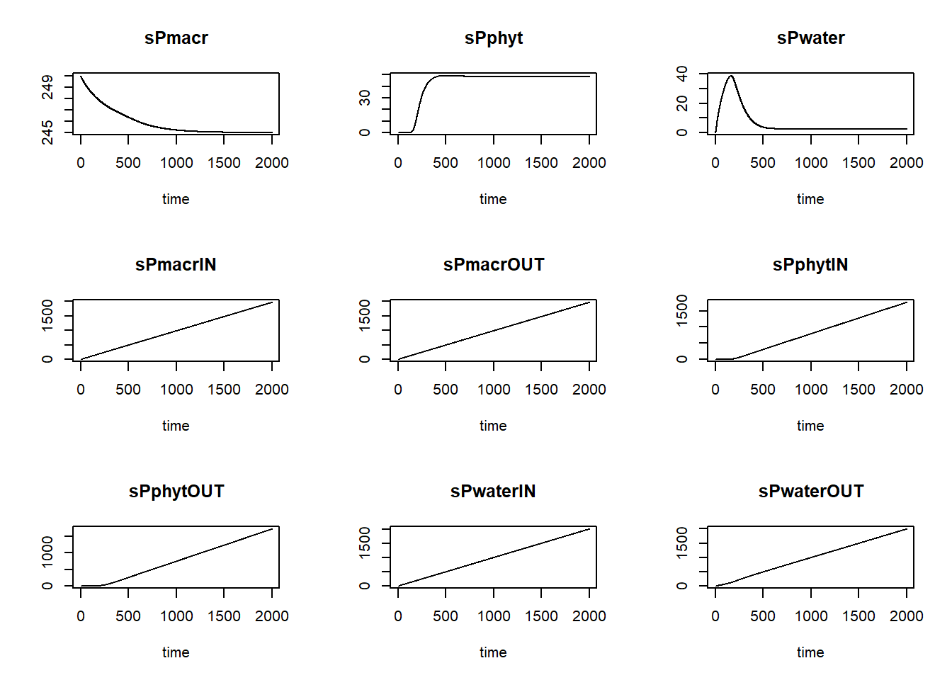

We can now define a function computing the mass balances, one that needs 2 inputs: state and init, which respectively are an object as returned by the ode function, and a vector with initial conditions for the state variables:

MassBalanceGPLakeR <- function(y, ini) {
  
  # Add "0" to the state variables' names to indicate initial condition
  names(ini) = paste0(names(ini), "0")
  
  # Using the with() function we can access elements directly by their name
  # here: 'y' is a deSolve matrix
  # so it is best to first convert it to a data.frame using function as.data.frame()
  # and then combine it with 'ini' using the function c()
  # and convert to a list using as.list()
  with(as.list(c(as.data.frame(y), ini)), {
    
    # Compute mass balance terms
    BAL = data.frame(time = time,
                     sPwaterbal = sPwater + sPwaterOUT - sPwaterIN - sPwater0,
                     sPmacrbal = sPmacr + sPmacrOUT - sPmacrIN - sPmacr0,
                     sPphytbal = sPphyt + sPphytOUT - sPphytIN - sPphyt0)

    # Return output BAL
    return(BAL)
  })
}

After defining this function, we can check the mass balances per state variable and plot them:

balance = MassBalanceGPLakeR(states, ini = InitGPLakeR())
par(mfrow = c(2,2))
plot(balance[,"time"], balance[,"sPwaterbal"], type="l", xlab="time", ylab="Balance sPwater")
plot(balance[,"time"], balance[,"sPmacrbal"], type="l", xlab="time", ylab="Balance sPmacr")
plot(balance[,"time"], balance[,"sPphytbal"], type="l", xlab="time", ylab="Balance sPphyt")
par(mfrow = c(1,1))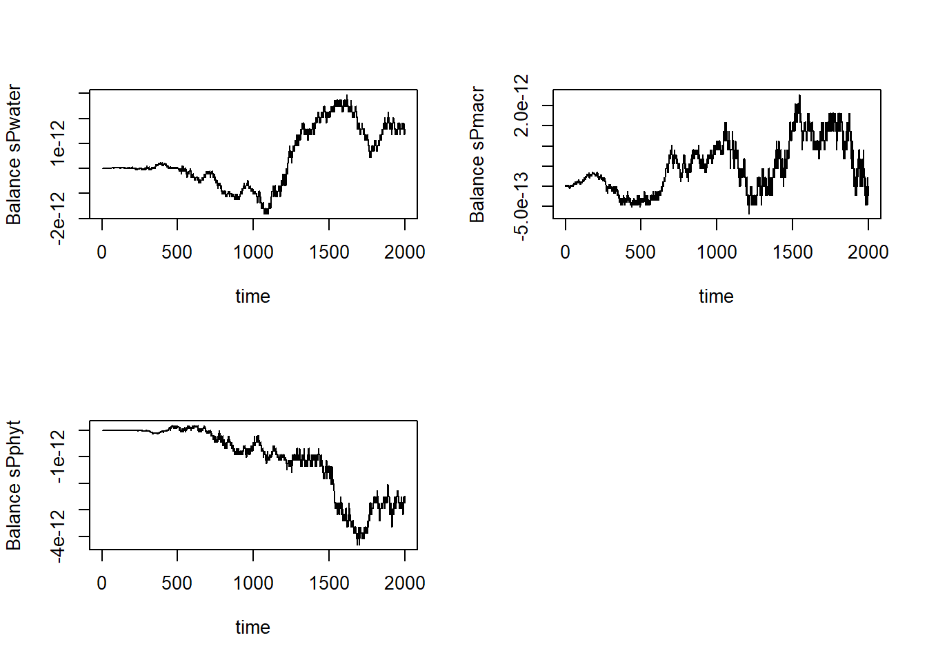

Note that the balances are sufficiently small (e.g. 1e-12) to consider it effectively zero!