Wageningen University & Research | FEM-31806 | Models for Ecological Systems | FEM | PPS | WEC
Template 6 - Calibration and evaluation
This is a code template that you can use as backbone for an R script that implements a model into code in order to solve it numerically, including methods to calibrate a model’s parameters and assess model fit.
Code template
A file containing the code template as shown in the code chunk below
can be downloaded
here. Places
indicated by ... need to be filled out (other parts of the
template consist of explanation, and include placeholders for parts that
will be completed in later lectures and templates):
# Template 6 - Calibration and evaluation
# See: https://wec.wur.nl/mes for explanation and examples

# Load the deSolve library
library(deSolve)

# Define a function that returns a named vector with initial state values
# see Template 1

# Define a function that returns a named vector with parameter values
# see Template 1

# Define a function for the rates of change of the state variables with respect to time
# see Template 1

# Define a function that computes prediction errors
# NOTE: nothing needs to be filled in here, so this function can be used as-is
# (unless there is a need to change it, e.g. change the solver method, or include events etc.)
predictionError <- function(p,          # the parameters
                            y0,         # the initial conditions
                            fn,         # the function with rate equation(s)
                            name,       # the name of the state parameter
                            obs_values, # the measured state values
                            obs_times,  # the time-points of the measured state values
                            out_time = seq(from = 0, # times for the numerical integration
                                           to = max(obs_times), # default: 0 - max(obs_times)
                                           by = 1) # in steps of 1
                            ) {
  # Get out_time vector to retrieve predictions for (combining 'obs_times' and 'out_time')
  out_time <- unique(sort(c(obs_times, out_time)))

  # Solve the model to get the prediction
  pred <- ode(y = y0,
              times = out_time,
              func = fn,
              parms = p,
              method = "ode45")
  # NOTE: in case of a 'stiff' problem, method "ode45" might result in an error that the max nr of
  # iterations is reached. Using method "rk4" (fixed timestep 4th order Runge-Kutta) might solve this.

  # Get predictions for our specific state, at times t
  pred_t <- subset(pred, time %in% obs_times, select = name)

  # Compute errors, err: prediction - obs
  err <- pred_t - obs_values

  # Return
  return(err)
}

# Define a function that computes the Root Mean Squared Error, RMSE
# NOTE: nothing needs to be filled in here, so this function can be used as-is
predRMSE <- function(...) { # NOTE: these ... are ellipsis, so DO NOT fill in something here!
  # Get prediction errors
  err <- predictionError(...) # NOTE: these ... are ellipsis, so DO NOT fill in something here!

  # Compute the measure of model fit (here the Root Mean Squared Error)
  RMSE <- sqrt(mean(err^2))

  # Return the measure of model fit
  return(RMSE)
}

# Define a function that allows for transformation and back-transformation
# NOTE: nothing needs to be filled in here, so this function can be used as-is
transformParameters <- function(parm, trans, rev = FALSE) {
  # Check transformation vector
  trans <- match.arg(trans, choices = c("none","logit","log"), several.ok = TRUE)

  # Get transformation function per parameter
  if(rev == TRUE) {
    # Back-transform from real scope to parameter scope
    transfun <- sapply(trans, switch,
                       "none" = mean,
                       "logit" = plogis,
                       "log" = exp)
  }else {
    # Transform from parameter scope to real scope
    transfun <- sapply(trans, switch,
                       "none" = mean,
                       "logit" = qlogis,
                       "log" = log)
  }

  # Apply transformation function
  y <- mapply(function(x, f){f(x)}, parm, transfun)

  # Return
  return(y)
}

# Define a function that performs the calibration of specified parameters
# NOTE: nothing needs to be filled in here, so this function can be used as-is
calibrateParameters <- function(par,  # parameters
                                init, # initial state values
                                fun,  # function that returns the rates of change
                                stateCol, # name of the state variable
                                obs,  # observed values of the state variable
                                t,    # timepoints of the observed state values
                                calibrateWhich, # names of the parameters to calibrate
                                transformations, # transformation per calibration parameter
                                times = seq(from = 0, # times for the numerical integration
                                            to = max(t), # default: 0 - max(t)
                                            by = 1), # in steps of 1
                                ... # NOTE: these ... are ellipsis, so DO NOT fill in something here!
                                    # these are the optional extra arguments past on to optim()
                                ) {
  # check names of parameters that need calibration
  calibrateWhich <- match.arg(calibrateWhich, choices = names(par), several.ok = TRUE)

  # Create vector with transformations for all parameters (set to "none")
  tranforms <- rep("none", length(par))
  names(tranforms) <- names(par) # set the names of each transformation

  # Overwrite the elements for parameters that need calibration
  tranforms[calibrateWhich] <- transformations

  # Transform parameters
  par <- transformParameters(parm = par, trans = tranforms, rev = FALSE)

  # Get parameters to be estimated
  par_fit <- par[calibrateWhich]

  # Specify the cost function: the function that will be optimized for the parameters to be estimated
  costFunction <- function(parm_optim, parm_all,
                           init, fun, stateCol, obs, t,
                           times = t,
                           optimNames = calibrateWhich,
                           transf = tranforms,
                           ... # NOTE: these ... are ellipsis, so DO NOT fill in something here!
                           ) {
    # Gather parameters (those that are and are not to be estimated)
    par <- parm_all
    par[optimNames] <- parm_optim[optimNames]

    # Back-transform
    par <- transformParameters(parm = par, trans = transf, rev = TRUE)

    # Get RMSE
    y <- predRMSE(p = par, y0 = init, fn = fun,
                  name = stateCol, obs_values = obs, obs_times = t,
                  out_time = times)

    # Return
    return(y)
  }

  # Fit using optim
  fit <- optim(par = par_fit,
               fn =  costFunction,
               parm_all = par,
               init = init,
               fun = fun,
               stateCol = stateCol,
               obs = obs,
               t = t,
               times = times,
               ...) # NOTE: these ... are ellipsis, so DO NOT fill in something here!
                    # These are the optional additional arguments passed on to optim()

  # Gather parameters: all parameters updated with those that are estimated
  y <- par
  y[calibrateWhich] <- fit$par[calibrateWhich]

  # Back-transform
  y <- transformParameters(parm = y, trans = tranforms, rev = TRUE)

  # put all (constant and estimated) parameters back in $par
  fit$par <- y

  # Add the calibrateWhich information
  fit$calibrated <- calibrateWhich

  # return 'fit'object:
  return(fit)
}

# Perform the calibration
fit <- calibrateParameters(par = ...,
                           init = ...,
                           fun = ...,
                           stateCol = ...,
                           obs = ...,
                           t = ...,
                           times = ...,
                           calibrateWhich = ...,
                           transformations = ...)
fit

# Fit the model using the calibrated values
statesFitted <- ode(y = ...,
                    times = ...,
                    parms = fit$par,
                    func = ...,
                    method = ...)
plot(statesFitted)
# etc, other ways of exploring/processing the fitted model
An example with explanation
Let’s continue with the example of Template 1, where we modelled a population with logistic growth:
with , and .
Model implementation
Because we already implemented this model already in Template 1, we can use the functions InitLogistic, ParmsLogistic and RatesLogistic as defined in Template 1.
Suppose we have measured data on the size of the population over time (column “t”):
surveyData <- data.frame(t = 0:50,
                         N = c(5,7,8,10,13,14,20,23,27,30,35,44,46,50,49,56,54,55,
                               57,56,58,62,58,54,47,47,42,47,48,48,51,54,51,43,36,
                               36,37,39,51,50,55,48,53,61,62,61,52,55,53,47,48))
plot(surveyData$t, surveyData$N, type = "l", xlab = "time", ylab = "population size")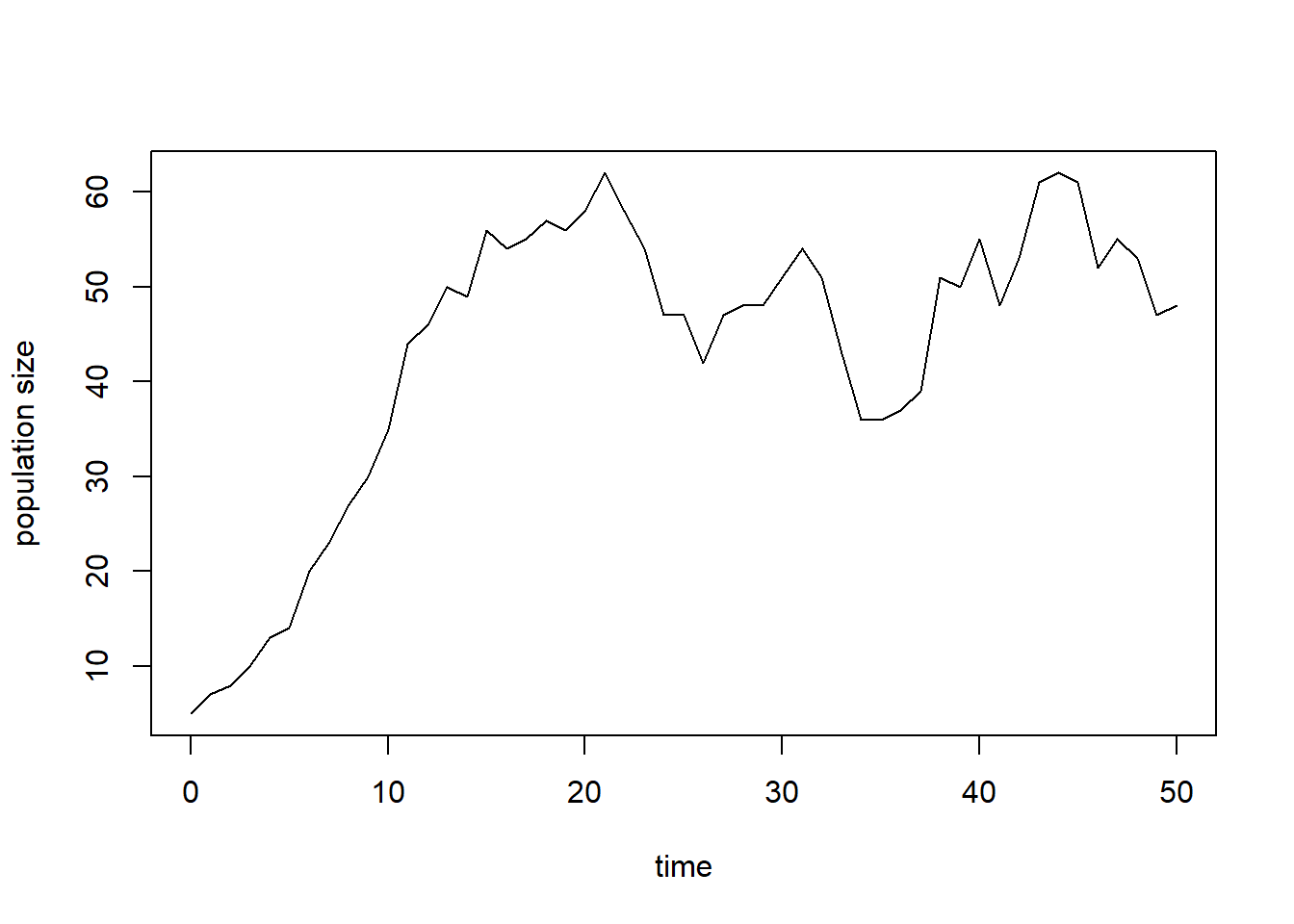
We can solve the model numerically using the above-mentioned parameter values and initial state values, after which we can plot the measured population density (points) as well as the predicted population size (line) as function of time:
states <- ode(y = InitLogistic(),
              times = surveyData$t,
              parms = ParmsLogistic(),
              func = RatesLogistic,
              method = "ode45")
plot(states[,"time"], states[,"N"], type = "l", xlab = "time", ylab = "N")
points(surveyData$t, surveyData$N)

# For clarity, let's add a legend:
legend(x = "topleft", bty = "n", lty = c(NA,1), pch = c(1,NA), legend = c("observation","prediction"))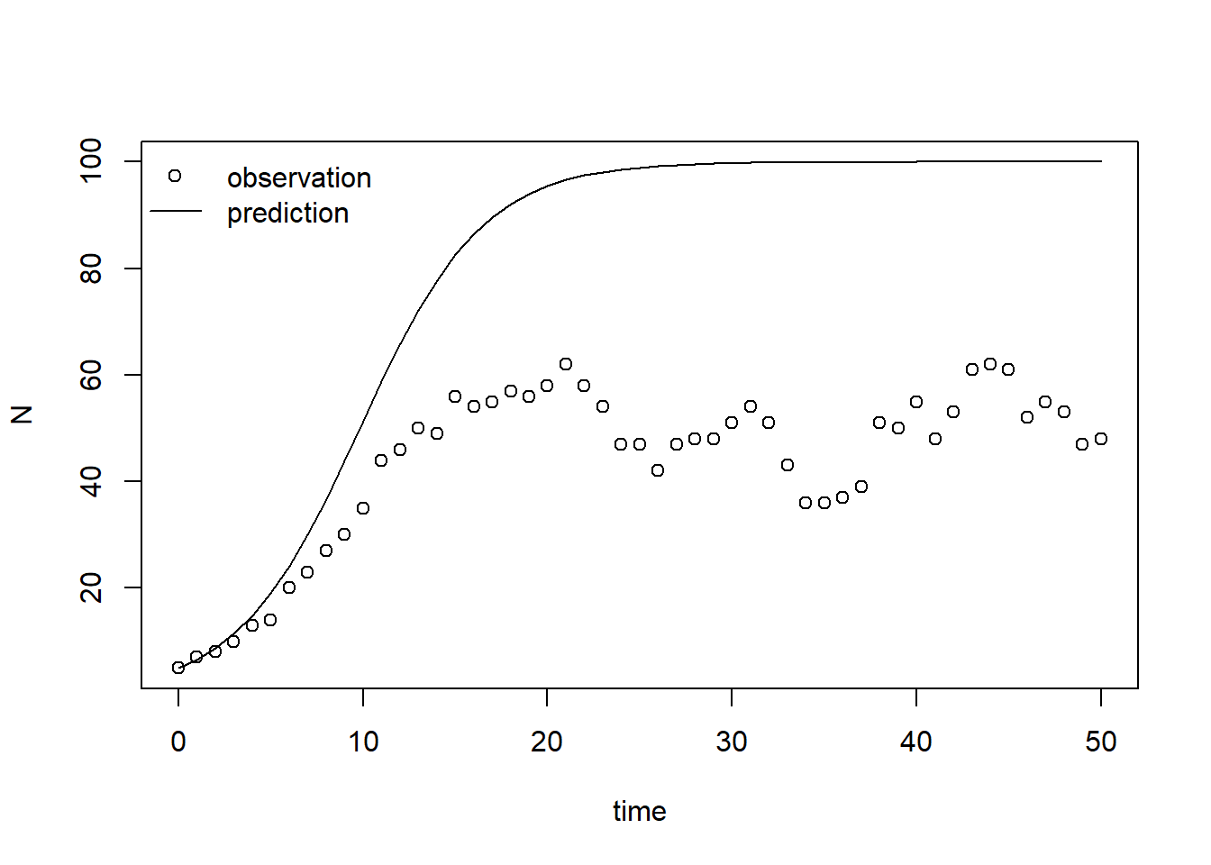
From this plot we can conclude that the model’s prediction does not agree with observations well. Thus, the set of parameter values does not seem to be calibrated well.
Quantifying prediction error
Model calibration and evaluation are both steps that depend on the
quantification of the prediction error: the difference between the
model’s predictions and the observed/measured values. Therefore, we will
define a function called predictionError that computes the
prediction error when given as input:
information to produce the model’s prediction:
p: the named vector of parameter values (i.e. the output of theParmsLogisticfunction);y0: the named vector of initial state values (i.e. the output of theInitLogisticfunction);fn: the function that returns the rates of change of the state variables (i.e. theRatesLogisticfunction);name: the name of the state variable for which to compute the prediction error (here it will be “N”);out_time: the times for which we want output (this determines the maximum timestep in the numerical simulation);
information on the measurements on the system:
obs_values: a set of observations/measurements of the state variable of interest;obs_times: the time-points where these observations were taken.
# Define a function that computes prediction errors
# NOTE: nothing needs to be filled in here, so this function can be used as-is
# (unless there is a need to change it, e.g. change the solver method, or include events etc.)
predictionError <- function(p,          # the parameters
                            y0,         # the initial conditions
                            fn,         # the function with rate equation(s)
                            name,       # the name of the state parameter
                            obs_values, # the measured state values
                            obs_times,  # the time-points of the measured state values
                            out_time = seq(from = 0, # times for the numerical integration
                                           to = max(obs_times), # default: 0 - max(obs_times)
                                           by = 1) # in steps of 1
                            ) {
  # Get out_time vector to retrieve predictions for (combining 'obs_times' and 'out_time')
  out_time <- unique(sort(c(obs_times, out_time)))

  # Solve the model to get the prediction
  pred <- ode(y = y0,
              times = out_time,
              func = fn,
              parms = p,
              method = "ode45")
  # NOTE: in case of a 'stiff' problem, method "ode45" might result in an error that the max nr of
  # iterations is reached. Using method "rk4" (fixed timestep 4th order Runge-Kutta) might solve this.

  # Get predictions for our specific state, at times t
  pred_t <- subset(pred, time %in% obs_times, select = name)

  # Compute errors, err: prediction - obs
  err <- pred_t - obs_values

  # Return
  return(err)
}
We can test the function by computing and plotting the prediction errors for the model relative to the observed values:
R <- predictionError(p = ParmsLogistic(),
                     y0 = InitLogistic(),
                     fn = RatesLogistic,
                     name = "N",
                     obs_values = surveyData$N,
                     obs_times = surveyData$t) # optionally add values for out_time
plot(surveyData$t, R, xlab = "time", ylab = "prediction error")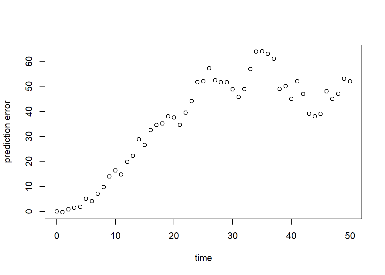
As we can see in both graphs above, the model (at its default parameter values!) systematically overestimates the observed population size. To have a single value summarizing this fit, we can compute a measure of model fit. Here, we compute the Root Mean Squared Error (RMSE; see table 8.1 in the syllabus):
sqrt(mean(R^2))## [1] 40.91814For this model parametrization, the RMSE is almost 41, and relative the average measured population size this is quite large!
Calibration
We thus proceed by calibrating the values of the model’s parameters. For this, we need to do a few things:
- First, we define a function that returns the RMSE when given the
same input as specified for the function
predictionErrorabove. Let’s call this functionpredRMSE. We will use the RMSE as the cost which should be optimized by a cost function in the optimization algorithm (theoptimfunction in R) that we will use for calibration. Often, optimization of the cost here means minimization: our objective in calibration is to find the set of parameter values that minimize the RMSE; - Second, we have to think carefully about the range of values that the parameters are allowed to have. In case of the logistic model described above, it is reasonable to assume and . Therefore, optimization algorithms that work best with unconstrained parameters (i.e., parameters that can have any value and ) cannot be used unless we transform the parameters first;
- Third, we thus need to transform the values prior to passing it on
to the optimization routine, and back-transform them inside our cost
function before calling function
predRMSE; - Fourth, once the optimization of the transformed parameters has been completed, we have to back-transform these parameters to their original scale.
Function predRMSE
Let’s start with the function for the RMSE, predRMSE. We
can define it as a simple function by using the ellipsis
... as the (only) input argument, and inside this function
we can pass it on to the function redictionError. Via the
ellipsis ... we can pass input arguments to the
predictionError function without having to explicitly
specify them in our definition of predRMSE. Obviously, we
could explicitly do so, but in this case this is a short and convenient
way to define our function. Thus: the predRMSE function
takes input via the ..., which it passes on to
predictionError, which returns the prediction errors. Then,
we compute the RMSE from these errors and return it:
# Define a function that computes the Root Mean Squared Error, RMSE
# NOTE: nothing needs to be filled in here, so this function can be used as-is
predRMSE <- function(...) { # NOTE: these ... are ellipsis, so DO NOT fill in something here!
  # Get prediction errors
  err <- predictionError(...) # NOTE: these ... are ellipsis, so DO NOT fill in something here!

  # Compute the measure of model fit (here the Root Mean Squared Error)
  RMSE <- sqrt(mean(err^2))

  # Return the measure of model fit
  return(RMSE)
}
Let’s test whether this function works:
predRMSE(p = ParmsLogistic(),
         y0 = InitLogistic(),
         fn = RatesLogistic,
         name = "N",
         obs_value = surveyData$N,
         obs_times = surveyData$t) # optionally add values for out_time
## [1] 40.91814Indeed, the value is similar to what we computed above (as it should be)!
Transformations
For the transformations and back-transformations, we have coded a simple function for you to facilitate these steps. This function allows for 3 types of transformations, which are among the most common types of transformations used (but there are more):
- “none”: no transformation, we simply leave the parameter value as-is. This should be the case for model parameters that can have any value and
- “log”: logarithmic transformation: this is a good transformation for parameters whose support is (e.g. the and parameters in our logistic growth model);
- “logit”: logit transformation: this is a convenient transformation for parameters whose support is and (e.g. fractions or probabilities).
The function is called transformParameters and takes as
input:
parm: the vector with parameters, e.g., a vector as returned by theParmsLogisticfunction;trans: a character vector with transformations: it should be of the same length as the parameter vector, and possible values for each parameter are “none”, “log” and “logit”.rev: a logical value (i.e.,TRUEorFALSE), specifying whether or not we and the back-transformation. IfFALSE, we transform the parameter from its own scope to unconstrained scope; ifTRUEwe back-transform from the unconstrained scale to the parameter scale:
# Define a function that allows for transformation and back-transformation
# NOTE: nothing needs to be filled in here, so this function can be used as-is
transformParameters <- function(parm, trans, rev = FALSE) {
  # Check transformation vector
  trans <- match.arg(trans, choices = c("none","logit","log"), several.ok = TRUE)

  # Get transformation function per parameter
  if(rev == TRUE) {
    # Back-transform from real scope to parameter scope
    transfun <- sapply(trans, switch,
                       "none" = mean,
                       "logit" = plogis,
                       "log" = exp)
  }else {
    # Transform from parameter scope to real scope
    transfun <- sapply(trans, switch,
                       "none" = mean,
                       "logit" = qlogis,
                       "log" = log)
  }

  # Apply transformation function
  y <- mapply(function(x, f){f(x)}, parm, transfun)

  # Return
  return(y)
}
Let’s test this function for our logistic growth model, for
parameters and , both via a “log” transform, and with
values as defined by function ParmsLogistic:
prm_t <- transformParameters(parm = ParmsLogistic(), trans = c("log","log"), rev = FALSE)
prm_t
## r K
## -1.203973 4.605170We can now easily back-transform the transformed parameter values (as
stored in object prm_t) with the same function using the
argument rev = TRUE:
prm_t_back <- transformParameters(parm = prm_t, trans = c("log","log"), rev = TRUE)
prm_t_back
## r K
## 0.3 100.0Indeed, after transformation and back-transformation, the parameter values are back to their original value: and .
Optimization function
We have predefined a function that allows you to do the optimization
when supplied with the needed data. The function needs all the inputs
that the predictionError function needs (see them described
above), but also 2 additional function inputs:
- “calibrateWhich”: a character vector with the names of the
parameters that are to be calibrated. This vector needs to be at least
of length 2 (otherwise the
optimfunction will not work), but you can choose to only select a subset of the model’s parameters for calibration; - “transformations”: a character vector with the transformation for
each model parameter (see above in the description of function
transformParameters).
Optionally, you can supply additional inputs to the
optim function via the three dots ellipsis
argument ... (e.g. when the calibration does not converge
within the default 500 iterations, you can then pass a higher number of
iteration as input to optim via argument
control, e.g. adding
control = list(maxit = 1000) increases the number of
iterations to 1000):
# Define a function that performs the calibration of specified parameters
# NOTE: nothing needs to be filled in here, so this function can be used as-is
calibrateParameters <- function(par,  # parameters
                                init, # initial state values
                                fun,  # function that returns the rates of change
                                stateCol, # name of the state variable
                                obs,  # observed values of the state variable
                                t,    # timepoints of the observed state values
                                calibrateWhich, # names of the parameters to calibrate
                                transformations, # transformation per calibration parameter
                                times = seq(from = 0, # times for the numerical integration
                                            to = max(t), # default: 0 - max(t)
                                            by = 1), # in steps of 1
                                ... # NOTE: these ... are ellipsis, so DO NOT fill in something here!
                                    # these are the optional extra arguments past on to optim()
                                ) {
  # check names of parameters that need calibration
  calibrateWhich <- match.arg(calibrateWhich, choices = names(par), several.ok = TRUE)

  # Create vector with transformations for all parameters (set to "none")
  tranforms <- rep("none", length(par))
  names(tranforms) <- names(par)

  # Overwrite the elements for parameters that need calibration
  tranforms[calibrateWhich] <- transformations

  # Transform parameters
  par <- transformParameters(parm = par, trans = tranforms, rev = FALSE)

  # Get parameters to be estimated
  par_fit <- par[calibrateWhich]

  # Specify the cost function: the function that will be optimized for the parameters to be estimated
  costFunction <- function(parm_optim, parm_all,
                           init, fun, stateCol, obs, t,
                           times = t,
                           optimNames = calibrateWhich,
                           transf = tranforms,
                           ... # NOTE: these ... are ellipsis, so DO NOT fill in something here!
                           ) {
    # Gather parameters (those that are and are not to be estimated)
    par <- parm_all
    par[optimNames] <- parm_optim[optimNames]

    # Back-transform
    par <- transformParameters(parm = par, trans = transf, rev = TRUE)

    # Get RMSE
    y <- predRMSE(p = par, y0 = init, fn = fun,
                  name = stateCol, obs_values = obs, obs_times = t,
                  out_time = times)

    # Return
    return(y)
  }

  # Fit using optim
  fit <- optim(par = par_fit,
               fn =  costFunction,
               parm_all = par,
               init = init,
               fun = fun,
               stateCol = stateCol,
               obs = obs,
               t = t,
               times = times,
               ...) # NOTE: these ... are ellipsis, so DO NOT fill in something here!
                    # These are the optional additional arguments passed on to optim()

  # Gather parameters: all parameters updated with those that are estimated
  y <- par
  y[calibrateWhich] <- fit$par[calibrateWhich]

  # Back-transform
  y <- transformParameters(parm = y, trans = tranforms, rev = TRUE)

  # put all (constant and estimated) parameters back in $par
  fit$par <- y

  # Add the calibrateWhich information
  fit$calibrated <- calibrateWhich

  # return 'fit'object:
  return(fit)
}
We have now defined all the necessary components needed for
calibration, so let’s calibrate the model parameters and
based on the data as defined in surveyData, and check the
output:
fit <- calibrateParameters(par = ParmsLogistic(),
                           init = InitLogistic(),
                           fun = RatesLogistic,
                           stateCol = "N",
                           obs = surveyData$N,
                           t = surveyData$t,
                           times = seq(from = 0, to = 50, by = 1),
                           calibrateWhich = c("r","K"),
                           transformations = c("log","log"))
fit
## $par
## r K
## 0.3291443 51.1938939
##
## $value
## [1] 6.262373
##
## $counts
## function gradient
## 65 NA
##
## $convergence
## [1] 0
##
## $message
## NULL
##
## $calibrated
## [1] "r" "K"What the function returns is a list with elements:
- “par”: the calibrated parameter values. This includes all model parameters: those that are kept constant as well as those that have been calibrated. Here the calibrated parameters are approximately and ;
- “value”: this is the value of the cost-function at the values as given in “par”. Here, this is thus the RMSE of the model predictions given the parameter values in “par”;
- “counts”: information about the number of iterations that the
optimfunction needed; - “convergence”: information about the convergence of the
optimfunction: a value of 0 means that the estimation successfully converged! For other values, see?optimfor the help-documentation of theoptimfunction; - “message”: a character string giving any additional information
returned by the optimizer, or
NULL; - “calibrated”: a character string with the model parameters that have
been calibrated (thus the vector passed as input to argument
calibrateWhich).
Using the calibrated parameter values, we can predict the state’s dynamics:
statesFitted <- ode(y = InitLogistic(),
                    times = surveyData$t,
                    parms = fit$par,
                    func = RatesLogistic,
                    method = "ode45")
# Plot the results
plot(surveyData$t, surveyData$N, xlab = "time", ylab = "N")
lines(statesFitted[,"time"], statesFitted[,"N"], col = 2, lwd = 2)
# For clarity, let's add a legend:
legend(x="topleft", bty = "n", lty = c(NA,1), pch = c(1,NA), legend = c("observation","prediction"))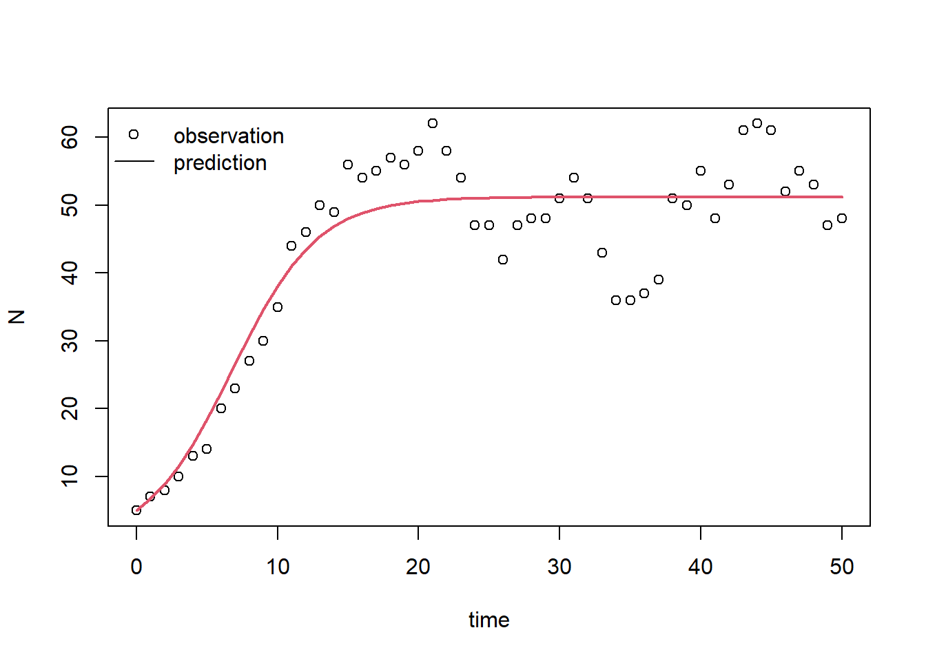
And, we can compute the RMSE for the calibrated model:
predRMSE(p = fit$par,
         y0 = InitLogistic(),
         fn = RatesLogistic,
         name = "N",
         obs_values = surveyData$N,
         obs_times = surveyData$t) # optionally add values for out_time
## [1] 6.262373Indeed, the model performs much better now! The RMSE decreased from 40.92 to 6.26!
Note that this last step is not a proper evaluation of the calibrated model! Namely, for that we would need an independent dataset.
Downloadable R script
An R script with the code chunks of the above example can be downloaded here.