Initial state variables

We first define a function that returns a named vector with initial state values, let’s call it InitLogistic4. We can copy InitLogistic from Template 1 - ODE basics in R. Because it is often useful to keep track of mass balances, let’s update the function by adding 2 state variables, “IN” and “OUT”, both with the initial value 0, so that we can keep track of the inputs and outputs in the system. Because at the start of a simulation both should have a value 0, we do not need to include “IN” and “OUT” in the function arguments, but rather can define them (with value 0) hard-coded in the function body!

InitLogistic4 <- function(N = 5) {
  # Gather function arguments in a named vector
  y <- c(N = N,   # population size
         IN = 0,  # sum of inputs
         OUT = 0) # sum of outputs
  
  # Return the named vector
  return(y)
}

To check, let’s run:

InitLogistic4()

##   N  IN OUT 
##   5   0   0

Note that we now have specified that there are 3 state variables (called “N”, “IN” and “OUT”), the function for the rates of change of the state variables (that we will specify below) should return the rate of change of all 3 specified states!

Parameter values

Because the model parameters have not changed compared to the function ParmsLogistic in Template 1, let’s copy that function and call it ParmsLogistic4.

ParmsLogistic4 <- function(r = 0.3, # intrinsic population growth rate
                           K = 100  # carrying capacity
                           ) {
  # Gather function arguments in a named vector
  y <- c(r = r,
         K = K)
  
  # Return the named vector
  return(y)
}

Rates of change

We can adapt the function RatesLogistic given in Template 1 to add some lines of code to keep track of the in and out flow so that we can compute mass balances, let’s call the new function RatesLogistic4:

RatesLogistic4 <- function(t, y, parms) {
  # use the with() function to be able to access the parameters and states easily
  # remember that the with() function is with(data, expr), where
  # - 'data' is ideally a list with named elements
  #   thus: 'y' and 'parms' are combined using function c and converted using function as.list
  # - 'expr' is an expression (i.e. code) that is evaluated
  #   this can span multiple lines of code when embraced with curly brackets {}
  with(
    as.list(c(y, parms)),{
      
      # Optional: forcing functions: get value of the driving variables at time t (if any)
      # see template 2
      
      # Optional: auxiliary equations

      # Rate equations
      dNdt <- r*N*(1-N/K)
      
      # Gather all rates of change in a vector
      # - the rates should be in the same order as the states (as specified in 'y')
      # - it can be a named vector, but does not need to be
      RATES <- c(dNdt = dNdt)
      
      # Optional: get in/out flow used to compute mass balances (or set MB <- NULL)
      dINdt <- r*N
      dOUTdt <- r*N*N/K
      MB <- c(dINdt = dINdt, dOUTdt = dOUTdt)

      # Optional: gather auxiliary variables that should be returned (or set AUX <- NULL)
      # - this should be a named vector or list!
      # here we pass the rate of change of N with respect to time back as auxiliary variable
      AUX <- RATES 
      
      # Return result as a list
      # - the first element is a vector with the rates of change (in the same order as 'y')
      # - all other elements are (optional) extra output, which should be named
      outList <- list(c(RATES, # the rates of change of the state variables
                        MB),   # the rates of change of the mass balance terms if MB is not NULL
                      AUX) # optional additional output per time step
      return(outList)
    }
  )
}

Solving the model

Because we will need the initial conditions both while solving the model, as well as when computing the mass balance checks, let’s store the initial conditions in an object called inits:

inits <- InitLogistic4()

Now we can solve the model, passing inits as input to argument y:

states <- ode(y = inits,
              times = seq(from = 0, to = 50, by = 1),
              func = RatesLogistic4,
              parms = ParmsLogistic4(),
              method = "ode45")

Mass balances

To check how the mass balance varies over time, we first need to specify a function that computes the mass balance as function of the solved model (states as computed above), as well as the initial state condition (object inits) as specified above. In this new function, let’s call it MassBalanceLogistic4, the solved model will be assigned to input argument y, and the initial state will be assigned to input argument ini. Within the function (also here using the with function to make it easier to access all initial states and columns in our solved model output directly by their name), we compute the mass balance (thus in this case the value of $N$ at any moment in time, minus $N_{t=0}$ plus the sum of outflows minus the sum of inflows):

MassBalanceLogistic4 <- function(y, ini) {
  # Add "0" to the state variables' names to indicate initial condition
  names(ini) = paste0(names(ini), "0")
  
  # Using the with() function we can access elements directly by there name
  # here: 'y' is a deSolve matrix
  # so it is best to first convert it to a data.frame using function as.data.frame()
  # and then combine it with 'ini' using the function c()
  # and convert to a list using as.list()
  with(as.list(c(as.data.frame(y), ini)), {
    
    # Compute mass balance terms
    BAL <- N - N0 + OUT - IN
    
    # Return output BAL
    return(BAL)
  })
}

After specifying this function, we can get the mass balance as a time series and plot to check it:

bal <- MassBalanceLogistic4(y = states, ini = inits)
plot(states[,"time"], bal, type = "l", xlab = "Time", ylab = "Mass balance")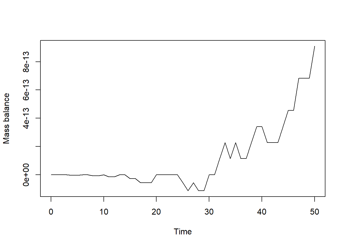

In the plot we see how the mass balance fluctuates over time. It is sufficiently small (1e-12 equals 0.000000000001!) and not exactly 0 due to the numerical approximation (and due to rounding error and the precision with which computers store data). Apart from this, the mass balance thus seems correct for this model!

Downloadable R script

An R script with the code chunks of the above example can be downloaded here.