Logistic growth

Let’s use the example of logistic growth as defined in Template 1, and include the objects that allow us to do mass balance checks (Template 4):

# Load the deSolve library
library(deSolve)

# Define a function that returns a named vector with initial state values
InitLogistic <- function(N = 5) {
  # Gather function arguments in a named vector
  y <- c(N = N,
         IN = 0,  # sum of inputs
         OUT = 0) # sum of outputs
  
  # Return the named vector
  return(y)
}

# Define a function that returns a named vector with parameter values
ParmsLogistic <- function(r = 0.3, # intrinsic population growth rate
                          K = 100 # carrying capacity
                          ){
  # Gather function arguments in a named vector
  y <- c(r = r,
         K = K)
  
  # Return the named vector
  return(y)
}

# Define a function for the rates of change of the state variables with respect to time
RatesLogistic <- function(t, y, parms) {
  # use the with() function to be able to access the parameters and states easily
  # remember that the with() function is with(data, expr), where
  # - 'data' is ideally a list with named elements
  #   thus: 'y' and 'parms' are combined using function c and converted using function as.list
  # - 'expr' is an expression (i.e. code) that is evaluated
  #   this can span multiple lines of code when embraced with curly brackets {}
  with(
    as.list(c(y, parms)), {
      
      # Optional: forcing functions: get value of the driving variables at time t (if any)
      # see template 2
      
      # Optional: auxiliary equations
      
      # Rate equations
      dNdt <- r*N*(1-N/K)
      
      # Gather all rates of change in a vector
      # - the rates should be in the same order as the states (as specified in 'y')
      # - it can be a named vector, but does not need to be
      RATES <- c(dNdt = dNdt)
      
      # Optional: get in/out flow used to compute mass balances (or set MB <- NULL)
      dINdt <- r*N
      dOUTdt <- r*N*N/K
      MB <- c(dINdt = dINdt, dOUTdt = dOUTdt)
      
      # Optional: gather auxiliary variables that should be returned (or set AUX <- NULL)
      # - this should be a named vector or list!
      AUX <- NULL
      
      # Return result as a list
      # - the first element is a vector with the rates of change (in the same order as 'y')
      # - all other elements are (optional) extra output, which should be named
      outList <- list(c(RATES, # the rates of change of the state variables
                        MB),   # the rates of change of the mass balance terms if MB is not NULL
                      AUX) # optional additional output per time step
      return(outList)
    }
  )
}

# Function to keep track of mass balances
MassBalanceLogistic <- function(y, ini){
  # Add "0" to the state variables' names to indicate initial condition
  names(ini) = paste0(names(ini), "0")
  
  # Using the with() function we can access elements directly by there name
  # here: 'y' is a deSolve matrix
  # so it is best to first convert it to a data.frame using function as.data.frame()
  # and then combine it with 'ini' using the function c()
  # and convert to a list using as.list()
  with(as.list(c(as.data.frame(y), ini)), {
    
    # Compute mass balance terms
    BAL <- N - N0 + OUT - IN
    
    # Return output BAL
    return(BAL)
  })
}

Mass balance checks

After defining these functions, we can solve the model, here without events, and perform a mass balance check:

# solve the model
states <- ode(y = InitLogistic(),
              times = seq(from = 0, to = 50, by = 0.1),
              func = RatesLogistic,
              parms = ParmsLogistic(),
              method = "ode45")

# mass balance check
bal <- MassBalanceLogistic(states, ini = InitLogistic())
plot(states[,"time"], bal, type = "l", xlab = "Time", ylab = "Mass balance")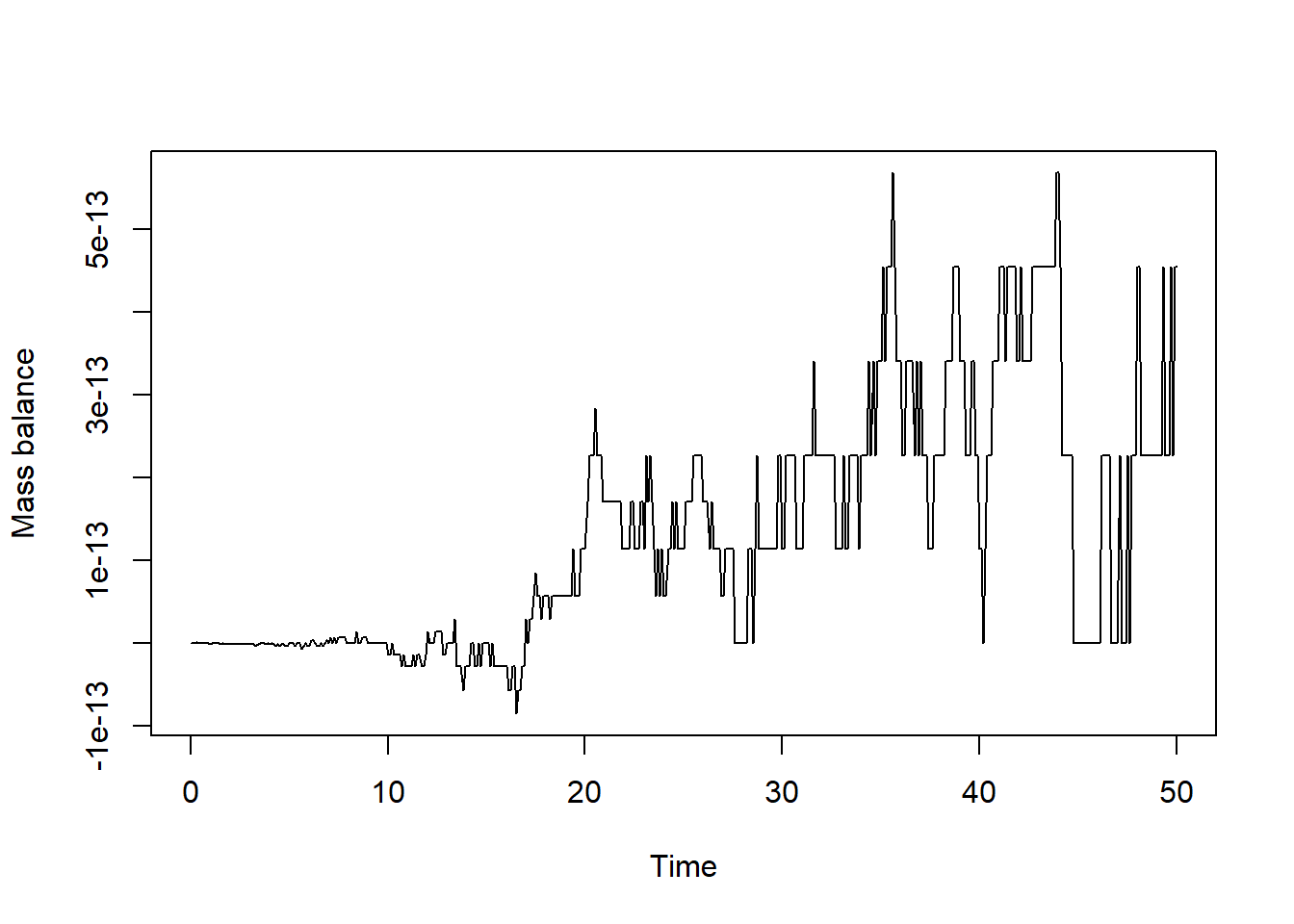

We see that the mass balance is (except for numerical inaccuracy) 0, so this is good!

Harvesting

As in Appendix A, let’s impose some harvesting of this population at pre-defined times: let’s remove 25% of the population at times 10, 20, 30 and 40: we do this via the specification of an event function that is applied at specified times:

# specify event function
eventfun <- function(t, y, parms){
  y["N"] <- 0.75 * y["N"]
  return(y)
}

# solve the model
states <- ode(y = InitLogistic(),
              times = seq(from = 0, to = 50, by = 0.1),
              func = RatesLogistic,
              parms = ParmsLogistic(),
              method = "ode45",
              events = list(func = eventfun, # the event function, called at times in "time"
                            time = c(10,20,30,40), # the time at which the event function is applied
                            root = FALSE)) # this specifies that we do not supply a root function
                                           # thus: the event function is called at the times supplied in "time"

# plot the simulation
plot(states)

# mass balance check
bal <- MassBalanceLogistic(states, ini = InitLogistic())
plot(states[,"time"], bal, type = "l", xlab = "Time", ylab = "Mass balance")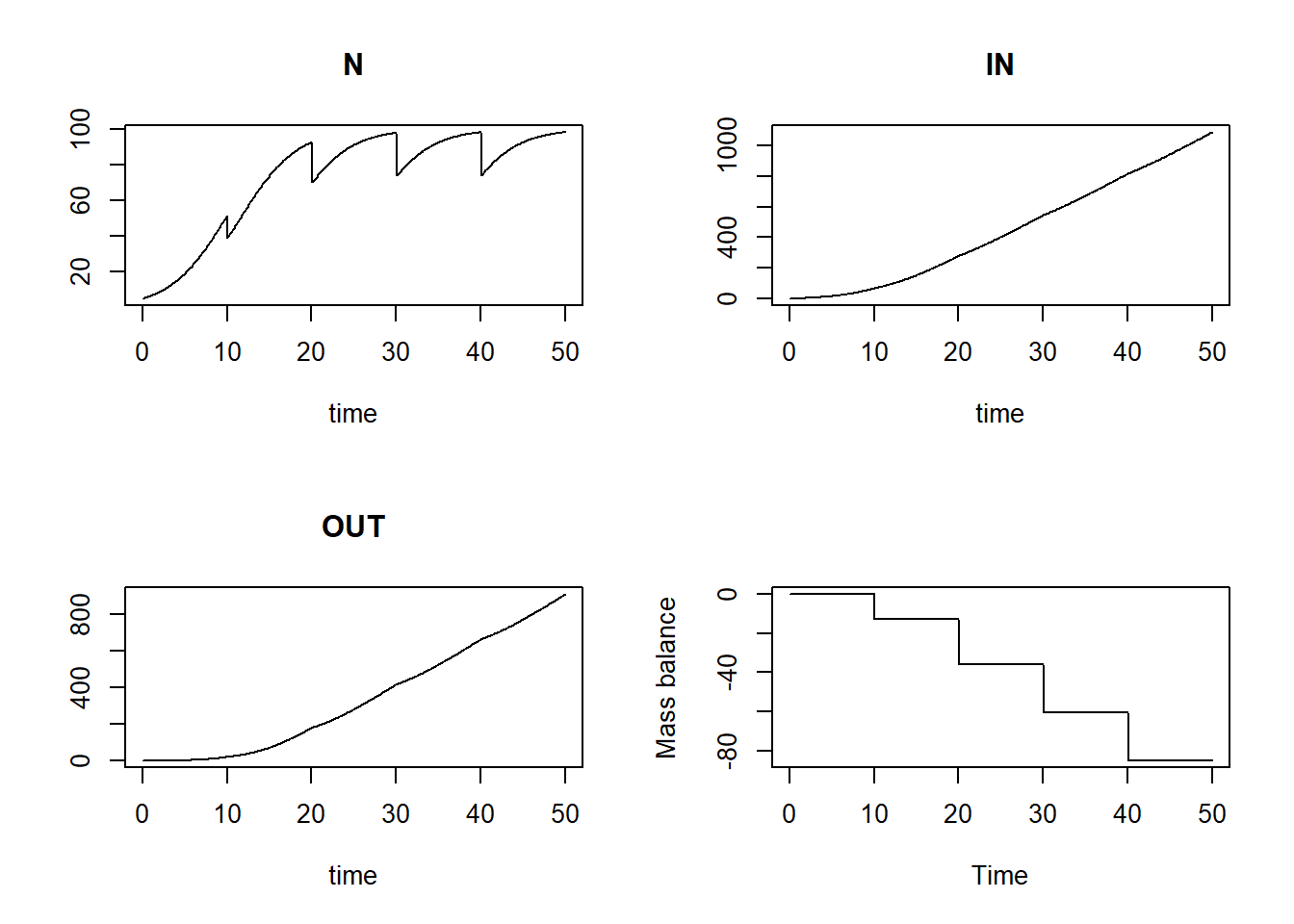

We see that the mass balance is not 0 anymore: we have partly harvested the population at specified times, but this is not considered in the mass balance check, therefore the mass balance is now wrong as it is not 0 anymore!

Mass balances when harvesting

In order to consider the discrete events acting on state variables in the mass balance check, we need to update the event function so that it also includes the influence of the event on the mass balance variables IN and OUT (depending on the type of event) as defined in the function InitLogistic. As we are dealing here with reduction of the state due to harvesting, we have to include the harvested part of the population in the rate of change for OUT.

Thus, in the event function eventfun, we first update the mass balance term OUT (i.e., we add 25% of state $N$ to the current value of OUT), after which we update the value of state $N$ (we remove 25% by multiplying it with 0.75):

# specify event function
eventfun <- function(t, y, parms){
  # first update OUT: add 25% of N to OUT
  y["OUT"] <- y["OUT"] + 0.25 * y["N"]
  
  # only then update N by removing 25%
  y["N"] <- 0.75 * y["N"]
  
  # return the updated version of vector y
  return(y)
}

# solve the model
states <- ode(y = InitLogistic(),
              times = seq(from = 0, to = 50, by = 0.1),
              func = RatesLogistic,
              parms = ParmsLogistic(),
              method = "ode45",
              events = list(func = eventfun, # the event function, called at times in "time"
                            time = c(10,20,30,40), # the time at which the event function is applied
                            root = FALSE)) # this specifies that we do supply a root function

# plot the simulation
plot(states)

# mass balance check
bal <- MassBalanceLogistic(states, ini = InitLogistic())
plot(states[,"time"], bal, type = "l", xlab = "Time", ylab = "Mass balance")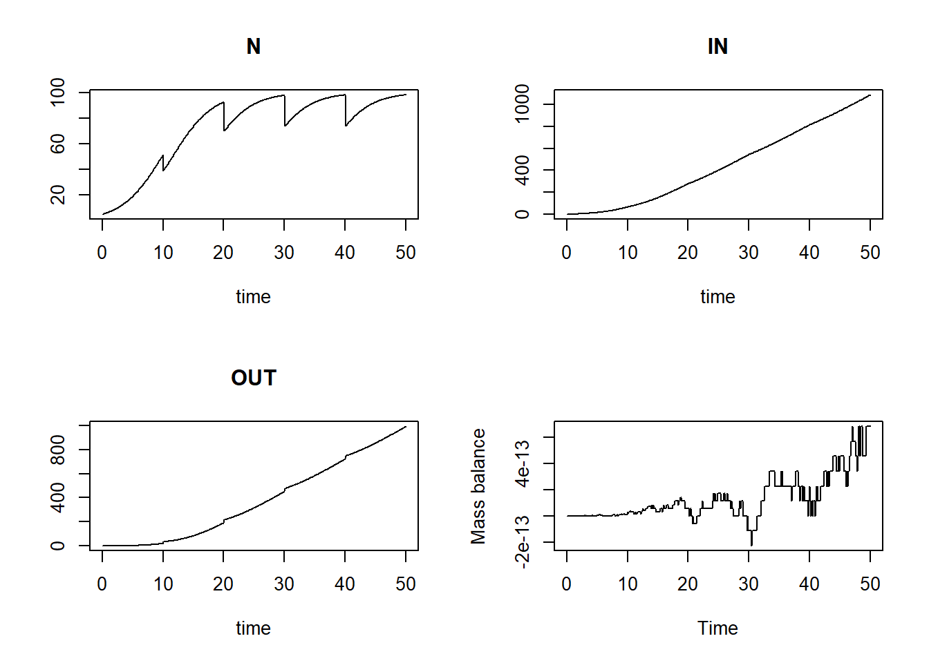

Now we see that the mass balance is again ca. 0 across the entire simulation, as it should!

Downloadable R script

An R script with the code chunks of the above example can be downloaded here.