Wageningen University & Research | FEM-31806 | Models for Ecological Systems | FEM | PPS | WEC
CO2Fix - Day 2
Aims
Implement the model
Implement the mini-Forest model in R. Use the equations as defined in the mini-model documents. Set up a basic structure to implement the model in R, using the provided R templates. Recall that this means defining (at least) 3 functions that will provide the main input to the
deSolveodefunction that will be used to numerically solve the model:- One function that defines the parameter values of the model: call
the function “ParmsCO2Fix”, this function will provide input to the
odeinput argumentparms; - One function that defines the initial values of the state variables
(call the function “InitCO2Fix”, this function will provide input to the
odeinput argumenty; - One function that defines the auxiliary variables and rates
equations for all states variables (call the function “RatesCO2Fix”,
this function will be the input to the
odeinput argumentfunc.
- One function that defines the parameter values of the model: call
the function “ParmsCO2Fix”, this function will provide input to the
Perform technical tests
Run the model for default parameters and initial state values. Check for any programming errors, including possible zero divisions or discontinuities. Ensure to run it for a sufficiently long period of time, e.g. 50 years, to check if the model reached an equilibrium or resulted in odd behaviour. Run the model using an adaptive stepsize Runge-Kutta integration method: method “ode45”.
Once there are no programming errors, plot the state variables against time: this helps for showing possible left errors. Importantly: does the simulation results reflect the intentions of the model developers?
Vary values of one key parameter. Before doing so, consider the possible effect of this on the state variable – time plots. Make the plots for the default model, but adapted for that single parameter value, and check whether the results follow your expectation. You can repeat this for another key parameter. If the model performs according your expectation, this gives further trust in the model.
Investigate the equilibria in your ecological system by evaluating the state variable – time plots. Does the system come in equilibrium? If not, try longer time periods for the simulation. Does the system ultimately come in equilibrium? If not, why not?
The rate of change of the state variable(s) should not change any longer in equilibrium. Plot therefore the state rates against time. Do these plots correspond with the state – time plots, and show the same results for equilibria?
Do you expect equilibria to differ (reach alternative stable states) when starting with different initial values? If so, vary initial values and check for existence of alternative equilibria.
Check if the computed values for state variables in equilibrium indeed result in rates with a value of 0, as additional check for the implemented formulas. Do this by filling in the computed results in the mathematical equations.
Analyse model behaviour for extreme values of some parameters. Does the model still run correctly, or will there be errors? Is the output what you expect?
Answers
Download here the code as shown on this page in a separate .r file.
Implement the model
See the Templates providing a structure to implement a model in R.
Parameters
The function returning a named vector with parameter values:
ParmsCO2fix <- function(
      ### External conditions
      IE = 200.0,  # IE external light intensity. If we consider the value of 200 and its
      # units of J PAR / (m2 s), this means for a day-length of 12 hours
      # 8.64 MJ / (m2 d). This is a reasonable value as an average over a
      # season, but the highest values during days of the season may reach
      # 30 MJ / (m2 d) or even more.
      CDGS = 200,  # CDGS days in a growing season, d/season, which is effectively d/y.
      CDLH = 12,   # CDLH sun hours in a day, hour/day = h/d.

      ### Tree specific parameters
      K = 0.7,     # K Light extinction coefficient (ranges from 0.5 - 0.9) m2 soil / (m2 leaf)
      SLA = 15.0,  # Specific Leaf Area (ranges from 10 - 20) m2 leaf / (kg leaf)
      FCL = 0.5,   # Fraction of C per mass of leaf: kgC / (kg of Leaf)
      LUE = 1.E-8, # Light use efficiency (ranges from 1.(08) - 4.3(2) gDW/MJ or
      # 0.001- 0.0043 kgDW/MJ), Sinclair and Muchow, 1999).
      # However, since the unit is here given in kg CO2 / (J PAR), the
      # range is between 1.8E-9 - 7.9E-9. The LUE is taken as 1.E-8,
      # which appears rather high.
      # Photosynthesis (PG), etc. are in terms of C(arbon), and the LUE should
      # also be given in gC/MJ. Assuming 50% of C per gram of dry matter
      # (DW) this would mean a value between 0.5 * (0.001- 0.0043 kgDW/MJ)
      # = 0.0005 - 0.0022 kgC/MJ.
      CF = 0.9,    # CF dimensionless curvature factor of the NRH or photosynthesis curve.
      PC = 1.E-6,  # PC photosynthesis capacity in kg CO2/(m2 s).

      # Allocation fractions: (kg assimilates to organ)/(kg assimilates produced by photosynthesis)
      NF = 0.2,      # constant allocation fraction of assimilates to foliage
      NS = 0.6,      # constant allocation fraction of assimilates to stem
      NR = 1 - (NF + NS), # The fraction to roots: 1 - fraction to (foliage+stem)

      # RF, RR and RS are (carbon) mass-based relative respiration rates for
      # F (foliage), R (roots) and S (shoot). Unit 1/year.
      RF = 0.1,
      RR = 0.1,
      RS = 0.1,
      # relative death rates or turnover rates, for
      # F (foliage), R (Roots), S (stem), and transition from sapwood to heartwood Unit 1/year.
      LRF = 1.0,
      LRR = 0.2,
      LRS = 0.05, # equal for sapwood and heartwood
      TSH = 0.1,

      ### Management related parameters
      NH = 0.1, # NH relative harvesting rate, 1/year, NP and NT: constant allocation
      # Unit NP       ; unit NT
      # (kgC of paper) (kgC of timber wood)
      # ------------- --------------------
      # (kgC of wood) (kgC of wood)
      NP = 0.2,   # fractions of harvested product to paper, NP, and timber, NT.
      NT = 1 - NP,# fractions of harvested product to timber
      LRP = 0.5,  # relative decay rates or turnover rates, for
      LRT = 0.02, # P (Paper) and T (Timber). Unit 1/year.
      LRW = 0.1   # loss rate waste
      # The inverse of these numbers gives the average residence time of the
      # product. If RGT=0.02, this means an average residence time of 50 years.
  ){

  # Constants, such as molecular weights. Constants must not be changed.
  MWC <- 12 # molar weight of C, g/mol
  MWO <- 16 # molar weight of O, g/mol
  # number of seconds per hour
  CSPH <- 3600

  # Gather parameters in a named vector
  y <- c(IE = IE, CDGS = CDGS, CDLH = CDLH, K = K, SLA = SLA,
         FCL = FCL, LUE = LUE, CF = CF, PC = PC,
         NF = NF, NS = NS, NR = NR,
         RF = RF, RR = RR, RS = RS, LRF = LRF, LRR = LRR, LRS = LRS, TSH = TSH,
         NH = NH, NP = NP, NT = NT, LRP = LRP, LRT = LRT, LRW = LRW,
         MWC = MWC, MWO = MWO, CSPH = CSPH)

  # Return
  return(y)
}
Initial conditions
The function returning a named vector with initial state values (all in units kgC m-2), here initialization according to the fractions that are allocated to the organs during the simulation:
InitCO2fix <- function(WF = 0.02, # WF, kgC in Foliage/m2
                       WR = 0.02, # WR, kgC in Roots/m2
                       WS = 0.06, # WS, kgC in Stems/m2
                       WH = 0.0,  # WH, kgC in Stems/m2
                       WP = 0.0,  # WP  kgC in paper/ m2
                       WT = 0.0,  # WT, kgC in timber/m2
                       WW = 0.0   # WW, kgC in waste/m2
                       ){
  # Gather initial conditions in a named vector; given names are names for the state variables in the model
  y <- c(WF = WF,
         WR = WR,
         WS = WS,
         WH = WH,
         WP = WP,
         WT = WT,
         WW = WW)

  # Return
  return(y)
}
Differential equations
The function computing the rates of change of the state variables with respect to time:
RatesCO2fix <- function(t, y, parms) {
  # use the with() function to be able to access the parameters and states easily
  # remember that the with() function is with(data, expr), where
  # - 'data' is ideally a list with named elements
  #   (thus combine 'y' and 'parms' first, using the function c(), then convert to list using as.list())
  # - 'expr' is an expression (i.e. code) that is evaluated
  #   this can span multiple lines of code when embraced with curly brackets {}
  with(
    as.list(c(y, parms)),{

      ### Optional: forcing functions: get value of the driving variables at time t (if any)

      ### Optional: auxiliary equations
      LAI <- WF * SLA / FCL
      IA <- IE *(1 - exp(-K * LAI ))

      PGS <- (1 / (2 * CF)) * (LUE * IA + PC -
                                 sqrt((LUE * IA + PC)^2 -4 * CF * LUE * IA* PC) )
      PG <- PGS * CSPH * CDLH * CDGS * (MWC / (MWC + 2 * MWO))
      PN <- PG - (RF * WF + RR * WR + RS * WS)

      ### Rate equations
      DWFDT <- PN * NF - LRF * WF - NH * WF
      DWRDT <- PN * NR - LRR * WR - NH * WR
      DWSDT <- PN * NS - LRS * WS - NH * WS - TSH*WS
      DWHDT <- TSH* WS - LRS * WH - NH * WH

      HT <- NH * (WF + WR + WS + WH) # total harvest
      HU <- NH * (WS + WH)           # useful harvest

      # The useful harvest, HU, is only the stem, so: (NH*DWS).
      # This is distributed over the two states paper and timber. These are
      # fractions of the useful harvest: paper NP; timber NT=(1-NP).
      DWPDT <- HU * NP - LRP * WP # paper
      DWTDT <- HU * NT - LRT * WT # Timber
      DWWDT <- HT - HU + LRF * WF + LRR * WR +LRS *(WS+WH) - LRW * WW # Waste

      ### Gather all rates of change in a vector
      # - the rates should be in the same order as the states (as specified in 'y')
      # - it can be a named vector, but does not need to be
      RATES <- c(DWFDT = DWFDT,
                 DWRDT = DWRDT,
                 DWSDT = DWSDT,
                 DWHDT = DWHDT,
                 DWPDT = DWPDT,
                 DWTDT = DWTDT,
                 DWWDT = DWWDT)

      ### Optional: get in/out flow used to compute mass balances (or set MB <- NULL)
      # not included here (thus here use MB <- NULL), see template 3
      MB <- NULL

      ### Optional: gather auxiliary variables that should be returned (or set AUX <- NULL)
      # - this should be a named vector or list!
      AUX <- NULL

      # Return result as a list
      # - the first element is a vector with the rates of change (in the same order as 'y')
      # - all other elements are (optional) extra output, which should be named
      outList <- list(c(RATES, # the rates of change of the state variables (same order as 'y'!)
                        MB),   # the rates of change of the mass balance terms (or NULL)
                      AUX) # optional additional output per time step
      return(outList)
    })
}
With these 3 functions now defined, the CO2Fix mini-model has been
implemented in R code, and the model can now numerically be solved using
the ode function from the deSolve package.
Performing technical tests
Use deSolve to integrate the model numerically using
Euler integration, here for 50 years in timesteps of 1:
states <- ode(y = InitCO2fix(),
              times = seq(from = 0, to = 50, by = 1),
              parms = ParmsCO2fix(),
              func = RatesCO2fix,
              method = "euler")
Model checks
We split up the testing of the model implementation in two steps: by checking whether the model runs technically and whether the computed results are reasonable.
First, if a model implementation runs technically without errors or important warning messages, it means e.g. that there are no zero divisions and no unexpected discontinuities. We can assess this by plotting state variables versus time or versus each other. If this appears to be correct, we can assess whether the model implementation computes results that are reasonable. First, we can plot the computed results using:
plot(states)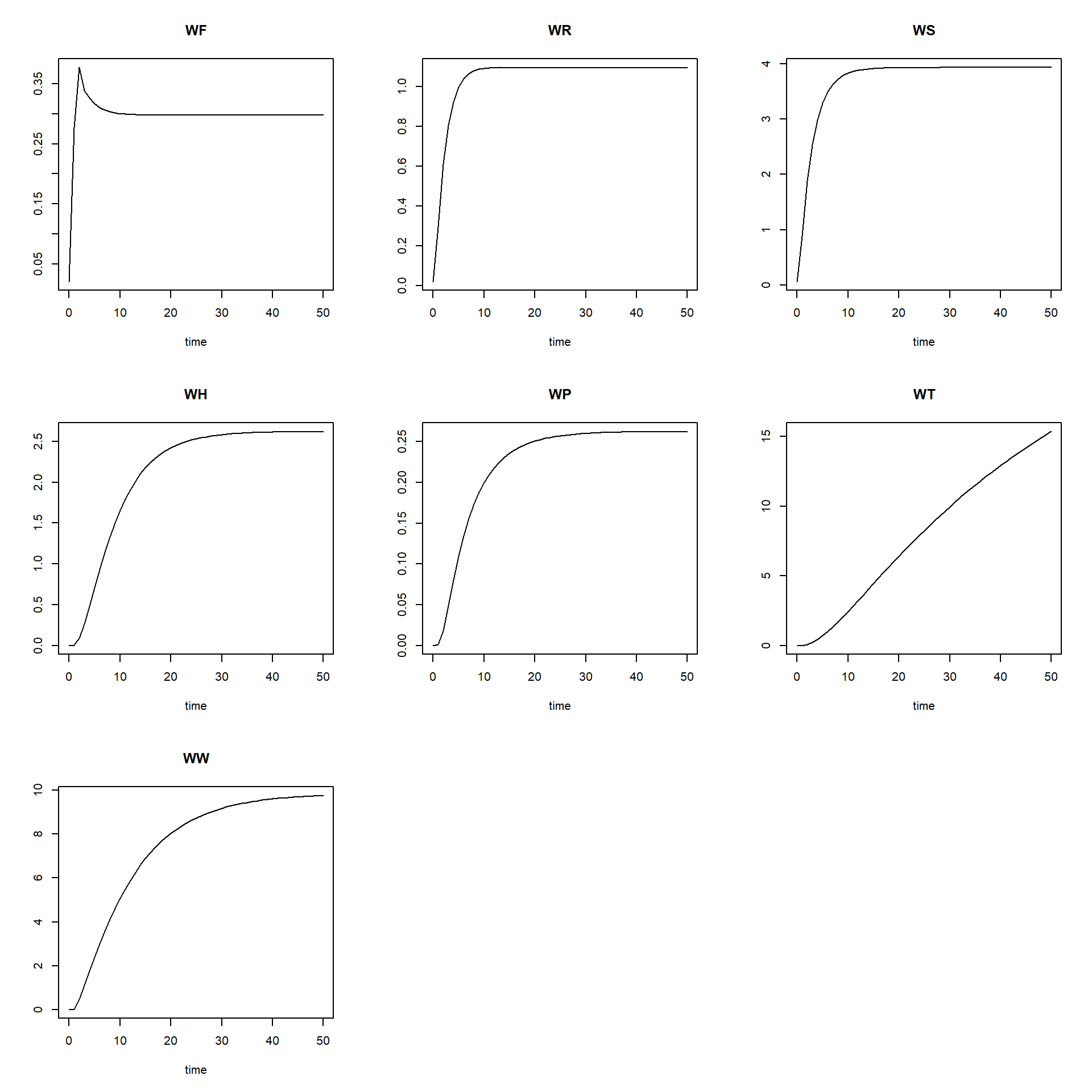
Second, we can check whether the results are reasonable by checking the units of the model implementation, similarly as for the model equations. Of course, if you did everything correctly, the units will be the same, but it is still needed and often programming errors are discovered. The reasonableness of results can also be checked if we know (or expect) that the model (and thus the model application) ought to reach an equilibrium. In that case the (net) rates will become zero. We can discover this by running the model for a long time period with small steps.
Some models will reach an equilibrium state after a period time. Often you have an expectation, if an equilibrium can be expected to occur.
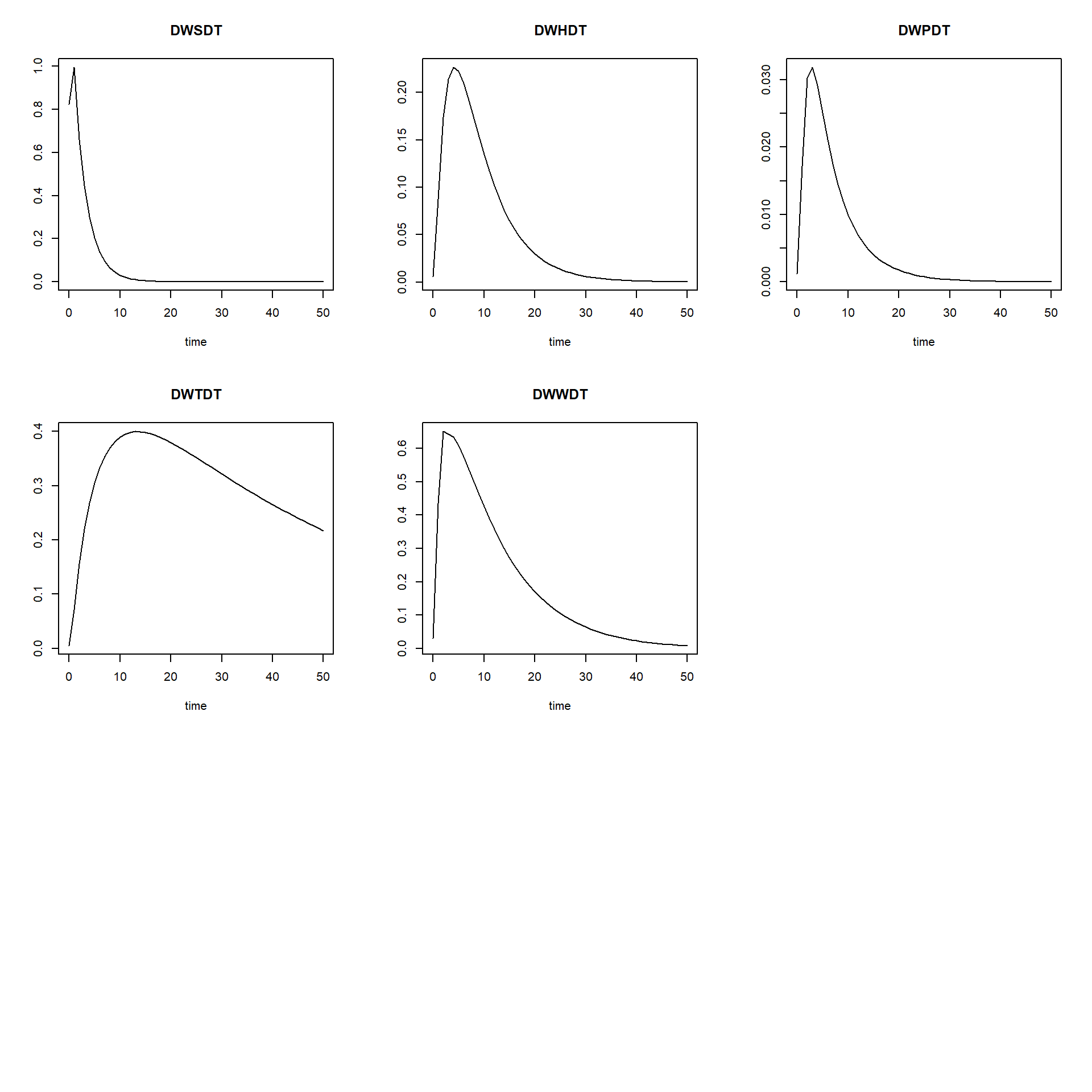
If we want to look at how the rates of change vary over time, and
thus not only the values of the state variables, we can do this easily
by changing AUX <- NULL into
AUX <- RATES in the function defined above that computes
the rates of change of the state variables. Then, simply running
plot(states) will not only plot the state variables as
function of time, but also their rates as function of time.
### SAME as earlier, but with AUX <- RATES
RatesCO2fix <- function(t, y, parms) {
  # use the with() function to be able to access the parameters and states easily
  # remember that the with() function is with(data, expr), where
  # - 'data' is ideally a list with named elements
  #   (thus combine 'y' and 'parms' first, using the function c(), then convert to list using as.list())
  # - 'expr' is an expression (i.e. code) that is evaluated
  #   this can span multiple lines of code when embraced with curly brackets {}
  with(
    as.list(c(y, parms)),{

      ### Optional: forcing functions: get value of the driving variables at time t (if any)

      ### Optional: auxiliary equations
      LAI <- WF * SLA / FCL
      IA <- IE *(1 - exp(-K * LAI ))

      PGS <- (1 / (2 * CF)) * (LUE * IA + PC -
                                 sqrt((LUE * IA + PC)^2 -4 * CF * LUE * IA* PC) )
      PG <- PGS * CSPH * CDLH * CDGS * (MWC / (MWC + 2 * MWO))
      PN <- PG - (RF * WF + RR * WR + RS * WS)

      ### Rate equations
      DWFDT <- PN * NF - LRF * WF - NH * WF
      DWRDT <- PN * NR - LRR * WR - NH * WR
      DWSDT <- PN * NS - LRS * WS - NH * WS - TSH*WS
      DWHDT <- TSH* WS - LRS * WH - NH * WH

      HT <- NH * (WF + WR + WS + WH) # total harvest
      HU <- NH * (WS + WH)           # useful harvest

      # The useful harvest, HU, is only the stem, so: (NH*DWS).
      # This is distributed over the two states paper and timber. These are
      # fractions of the useful harvest: paper NP; timber NT=(1-NP).
      DWPDT <- HU * NP - LRP * WP # paper
      DWTDT <- HU * NT - LRT * WT # Timber
      DWWDT <- HT - HU + LRF * WF + LRR * WR +LRS *(WS+WH) - LRW * WW # Waste

      ### Gather all rates of change in a vector
      # - the rates should be in the same order as the states (as specified in 'y')
      # - it can be a named vector, but does not need to be
      RATES <- c(DWFDT = DWFDT,
                 DWRDT = DWRDT,
                 DWSDT = DWSDT,
                 DWHDT = DWHDT,
                 DWPDT = DWPDT,
                 DWTDT = DWTDT,
                 DWWDT = DWWDT)

      ### Optional: get in/out flow used to compute mass balances (or set MB <- NULL)
      # not included here (thus here use MB <- NULL), see template 3
      MB <- NULL

      ### Optional: gather auxiliary variables that should be returned (or set AUX <- NULL)
      # - this should be a named vector or list!
      AUX <- RATES

      # Return result as a list
      # - the first element is a vector with the rates of change (in the same order as 'y')
      # - all other elements are (optional) extra output, which should be named
      outList <- list(c(RATES, # the rates of change of the state variables (same order as 'y'!)
                        MB),   # the rates of change of the mass balance terms (or NULL)
                      AUX) # optional additional output per time step
      return(outList)
    })
}

# solve the model
states <- ode(y = InitCO2fix(),
              times = seq(from = 0, to = 50, by = 1),
              parms = ParmsCO2fix(),
              func = RatesCO2fix,
              method = "euler")

# explore
head(states)
## time WF WR WS WH WP WT WW DWFDT DWRDT DWSDT DWHDT DWPDT DWTDT
## [1,] 0 0.0200000 0.0200000 0.0600000 0.00000000 0.00000000 0.00000000 0.0000000 0.257495098 0.27349510 0.8234853 0.00600000 0.00120000 0.00480000
## [2,] 1 0.2774951 0.2934951 0.8834853 0.00600000 0.00120000 0.00480000 0.0310000 0.099690951 0.31688703 0.9939354 0.08744853 0.01718971 0.07106282
## [3,] 2 0.3771860 0.6103821 1.8774206 0.09344853 0.01838971 0.07586282 0.4656674 -0.038035918 0.19375410 0.6612510 0.17372479 0.03022253 0.15615228
## [4,] 3 0.3391501 0.8041362 2.5386717 0.26717331 0.04861224 0.23201510 1.1156634 -0.012560376 0.11926390 0.4468464 0.21379117 0.03181078 0.21982730
## [5,] 4 0.3265898 0.9234001 2.9855181 0.48096449 0.08042302 0.45184240 1.7586953 -0.009828462 0.07240023 0.3018813 0.22640713 0.02911814 0.26828176
## [6,] 5 0.3167613 0.9958004 3.2873994 0.70737162 0.10954116 0.72012416 2.3924187 -0.006319573 0.04337774 0.2045037 0.22263419 0.02512484 0.30517920
## DWWDT
## [1,] 0.0310000
## [2,] 0.4346674
## [3,] 0.6499960
## [4,] 0.6430319
## [5,] 0.6337234
## [6,] 0.6076742plot(states)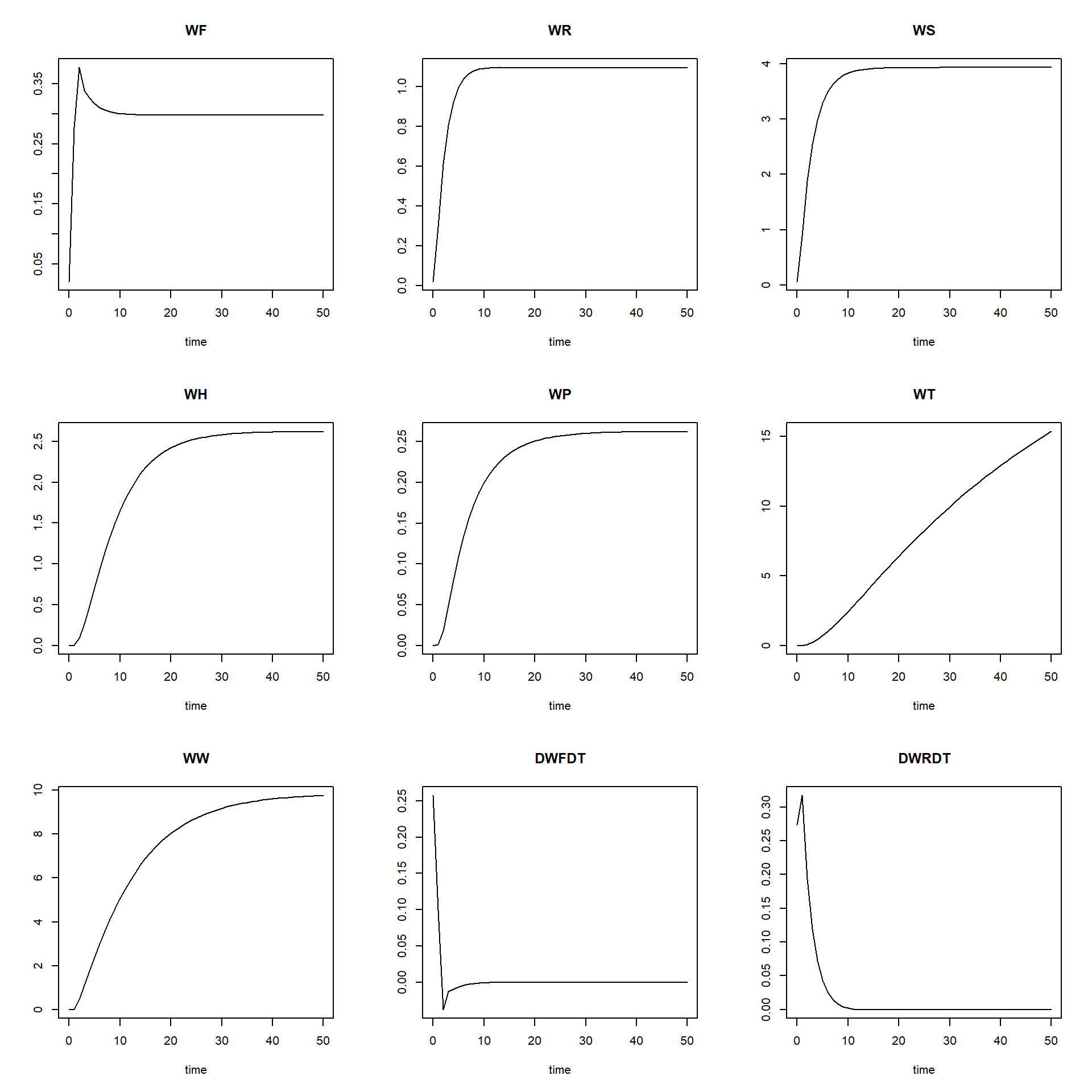
Moreover, we can easily change parameter values or initial state
values from their defaults, by including input values to the function
calls to functions “ParmsCO2Fix” (input to the argument
parms in the ode function call), as well as
function “InitCO2Fix” (input to the argument y in the
ode function call).