Wageningen University & Research | FEM-31806 | Models for Ecological Systems | FEM | PPS | WEC
CO2Fix - Day 3
Aims
Time step convergence
Compare different methods of integration for different time steps. Note that you can simply set these as arguments for your model calling function
ode. Compare the Euler method with a variable time-step 4th order Runga-Kutta method (“ode45”). Run the model with Euler for a time step of 1, 1.5 and 1.75 years. Save the output with computed states for these runs with Euler and save also one output for a run with ode45 as method. For a direct comparison with output at exactly the same moments in time for both integration methods, you can define the variabledeltand adjust the sequence that you use to define the output for time (e.g.:seq(0, 1000, by=delt)). Note that the actual time-steps taken by when using the ode45 integration method will be smaller as the time step is in this method adjusted when required.Plot the state variables of the 4 simulations against time in the same plot. Alternatively, plot the state variables of each of the three Euler simulations with those computed with the ode45 integration method in a plot. Limit the plotting ranges for the x- and y by setting
xlim = c(... , ...)andylim = c(... , ...)to zoom in to times when the model outputs quickly change. What can you roughly conclude for the appropriate time step using Euler?You can also calculate the relative deviation of Euler when compared to the ode45 results (by computing |Euler state-RK state|/RK state , for example at time = 50 years). Within what range of time-step values do state variables not differ more than 1% after a reasonable time period (50 years)?
Develop an equation to calculate the time coefficients for each of the state variables. Implement them and plot time coefficients against time.
Mass balances tests
- Choose the appropriate mass variables in your model, either C, P or N if present.
- Define the sum of all the mass inflows and all the sum of all mass outflows for each of your mass variables in the model.
- Define the balance for each of the mass variables in the model.
- Create a plot to check the mass balance visually: in other words, check the dynamics in each of the mass variables over time. What is your expectation? Is your expectation supported by the graphical output?
Answers
Download here the code as shown on this page in a separate .r file.
Compare integration methods
To check for the difference between Euler and Runge-Kutta
integration, let’s solve the model numerically for 50 time-units in
time-steps of 1, 1.5 and 1.75 (the fixed time-step of the
euler method), as well as with a variable time-step
Runge-Kutta method (ode45, here with output every
time-step):
states_rk <- ode(y = InitCO2fix(),
                 times = seq(from = 0, to = 50, by = 1),
                 parms = ParmsCO2fix(),
                 func = RatesCO2fix,
                 method = "ode45")

delt <- 1
states_euler1 <- ode(y = InitCO2fix(),
                     times = seq(from = 0, to = 50, by = delt),
                     parms = ParmsCO2fix(),
                     func = RatesCO2fix,
                     method = "euler")

delt <- 1.5
states_euler2 <- ode(y = InitCO2fix(),
                     times = seq(from = 0, to = 50, by = delt),
                     parms = ParmsCO2fix(),
                     func = RatesCO2fix,
                     method = "euler")

delt <- 1.75
states_euler3 <- ode(y = InitCO2fix(),
                     times = seq(from = 0, to = 50, by = delt),
                     parms = ParmsCO2fix(),
                     func = RatesCO2fix,
                     method = "euler")
We can have a look at the output of the last time-steps (for all 4 solutions):
tail(states_rk)## time WF WR WS WH WP WT WW DWFDT DWRDT DWSDT DWHDT DWPDT DWTDT
## [46,] 45 0.2978606 1.092157 3.931755 2.615400 0.2617871 14.16006 9.657869 -2.135739e-08 -5.291068e-07 1.403259e-06 0.0008653870 4.954577e-05 0.2405713
## [47,] 46 0.2978606 1.092157 3.931756 2.616204 0.2618331 14.39827 9.673938 -1.584266e-08 -4.046576e-07 1.053836e-06 0.0007449584 4.264028e-05 0.2358714
## [48,] 47 0.2978606 1.092157 3.931757 2.616896 0.2618727 14.63183 9.688513 -1.176274e-08 -3.092030e-07 7.917345e-07 0.0006412765 3.669775e-05 0.2312557
## [49,] 48 0.2978606 1.092156 3.931757 2.617491 0.2619068 14.86081 9.701731 -8.741324e-09 -2.360721e-07 5.950428e-07 0.0005520155 3.158377e-05 0.2267237
## [50,] 49 0.2978606 1.092156 3.931758 2.618004 0.2619361 15.08530 9.713718 -6.501606e-09 -1.801030e-07 4.473731e-07 0.0004751721 2.718272e-05 0.2222749
## [51,] 50 0.2978606 1.092156 3.931758 2.618445 0.2619614 15.30539 9.724587 -4.839785e-09 -1.373092e-07 3.364623e-07 0.0004090204 2.339513e-05 0.2179086
## DWWDT
## [46,] 0.01686474
## [47,] 0.01529795
## [48,] 0.01387496
## [49,] 0.01258283
## [50,] 0.01140973
## [51,] 0.01034489tail(states_euler1)## time WF WR WS WH WP WT WW DWFDT DWRDT DWSDT DWHDT DWPDT DWTDT
## [46,] 45 0.2978606 1.092156 3.931759 2.617694 0.2619185 14.18879 9.688503 -2.153625e-09 -7.654115e-08 1.661031e-07 0.0005218025 2.982819e-05 0.2401804
## [47,] 46 0.2978606 1.092156 3.931759 2.618216 0.2619483 14.42897 9.702419 -1.537631e-09 -5.533180e-08 1.193183e-07 0.0004435487 2.535347e-05 0.2354186
## [48,] 47 0.2978606 1.092156 3.931759 2.618659 0.2619736 14.66439 9.714969 -1.098662e-09 -3.998469e-08 8.573146e-08 0.0003770284 2.155010e-05 0.2307457
## [49,] 48 0.2978606 1.092155 3.931759 2.619036 0.2619952 14.89514 9.726286 -7.855592e-10 -2.888471e-08 6.161232e-08 0.0003204827 1.831733e-05 0.2261609
## [50,] 49 0.2978606 1.092155 3.931759 2.619357 0.2620135 15.12130 9.736491 -5.620460e-10 -2.085990e-08 4.428743e-08 0.0002724164 1.556955e-05 0.2216634
## [51,] 50 0.2978606 1.092155 3.931759 2.619629 0.2620291 15.34296 9.745691 -4.023655e-10 -1.506050e-08 3.183986e-08 0.0002315584 1.323399e-05 0.2172519
## DWWDT
## [46,] 0.013915631
## [47,] 0.012550141
## [48,] 0.011317292
## [49,] 0.010204405
## [50,] 0.009199983
## [51,] 0.008293600tail(states_euler2)## time WF WR WS WH WP WT WW DWFDT DWRDT DWSDT DWHDT DWPDT DWTDT
## [29,] 42.0 0.2978599 1.092156 3.931759 2.616865 0.2618711 13.44663 9.655125 7.886133e-07 -3.533391e-08 1.664864e-07 0.0006461048 3.692642e-05 0.2549574
## [30,] 43.5 0.2978610 1.092156 3.931759 2.617834 0.2619265 13.82906 9.680941 -5.375396e-07 -4.437463e-08 2.923109e-08 0.0005007562 2.861975e-05 0.2473862
## [31,] 45.0 0.2978602 1.092155 3.931759 2.618586 0.2619694 14.20014 9.702960 3.641736e-07 -9.633215e-09 6.258793e-08 0.0003880905 2.217850e-05 0.2400247
## [32,] 46.5 0.2978608 1.092155 3.931759 2.619168 0.2620027 14.56018 9.721732 -2.480020e-07 -1.658745e-08 5.249897e-09 0.0003007795 1.718922e-05 0.2328706
## [33,] 48.0 0.2978604 1.092155 3.931759 2.619619 0.2620285 14.90949 9.737732 1.681475e-07 -2.176906e-09 2.411977e-08 0.0002331049 1.332085e-05 0.2259206
## [34,] 49.5 0.2978607 1.092155 3.931759 2.619969 0.2620485 15.24837 9.751365 -1.144331e-07 -6.334554e-09 -3.369122e-10 0.0001806599 1.032408e-05 0.2191709
## DWWDT
## [29,] 0.017211279
## [30,] 0.014679342
## [31,] 0.012514093
## [32,] 0.010666687
## [33,] 0.009088826
## [34,] 0.007743263tail(states_euler3)## time WF WR WS WH WP WT WW DWFDT DWRDT DWSDT DWHDT DWPDT DWTDT
## [24,] 40.25 0.3350770 1.092934 3.933870 2.615526 0.2617257 12.98520 9.587361 -0.04168243 -0.0009779823 -0.002760613 1.058181e-03 1.250792e-04 0.2642477
## [25,] 42.00 0.2621328 1.091223 3.929039 2.617377 0.2619446 13.44763 9.701458 0.03996850 0.0009477095 0.002683908 2.973015e-04 -4.395022e-05 0.2547607
## [26,] 43.75 0.3320777 1.092881 3.933736 2.617898 0.2618676 13.89346 9.654012 -0.03832255 -0.0009015249 -0.002545362 6.889438e-04 9.884857e-05 0.2462614
## [27,] 45.50 0.2650132 1.091304 3.929282 2.619103 0.2620406 14.32442 9.750840 0.03674931 0.0008727345 0.002471110 6.265765e-05 -5.261858e-05 0.2373824
## [28,] 47.25 0.3293245 1.092831 3.933606 2.619213 0.2619485 14.73984 9.700512 -0.03523849 -0.0008308293 -0.002346135 4.786543e-04 8.210455e-05 0.2294287
## [29,] 49.00 0.2676571 1.091377 3.929500 2.620051 0.2620922 15.14134 9.783980 0.03379382 0.0008035668 0.002274931 -5.756612e-05 -5.509876e-05 0.2211373
## DWWDT
## [24,] 0.06519874
## [25,] -0.02711211
## [26,] 0.05533027
## [27,] -0.02875917
## [28,] 0.04769601
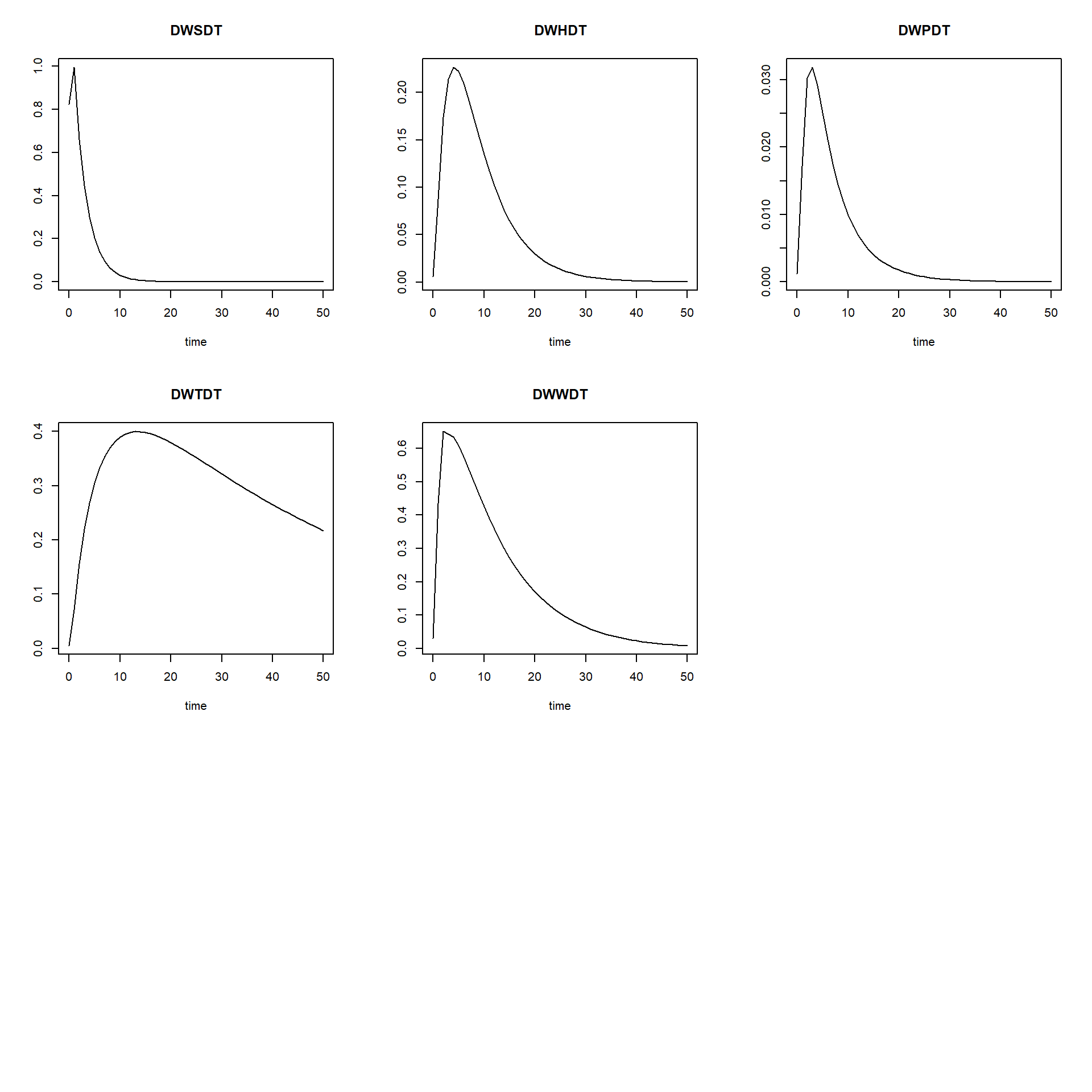
## [29,] -0.02908449Now, you can plot all solutions together in a single figure using:
plot(states_rk, states_euler1,states_euler2, states_euler3)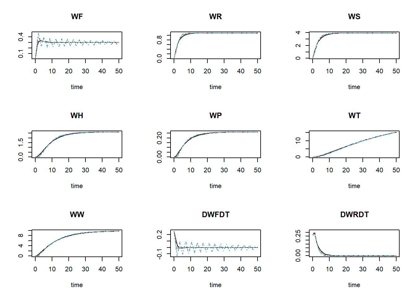
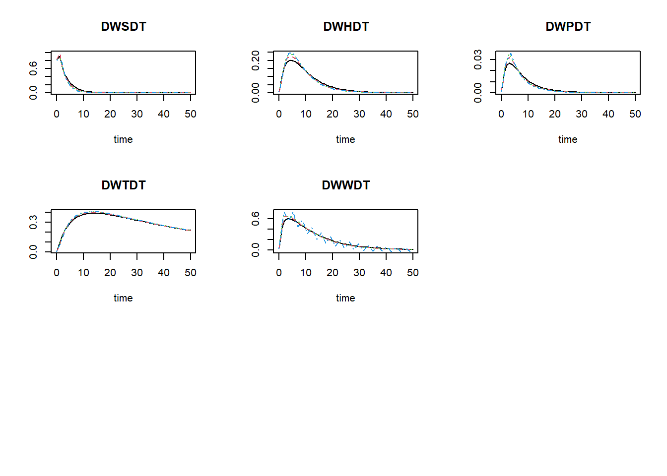
The black line now is the Runge-Kutta solution (with variable
time-step), the dashed red line is the first Euler solution (with
time-step of 1), the dashed green line is the second Euler solution
(with time-step of 1.5), and the dashed blue line is the third Euler
solution (with time-step of 1.75). To focus a bit more on the first time
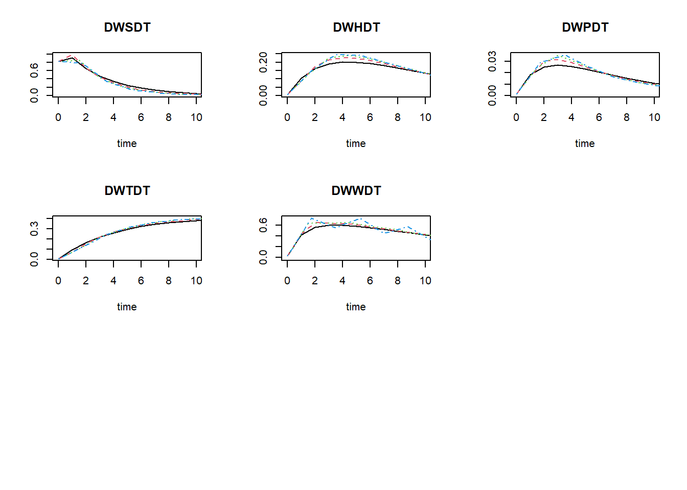
steps, we can limit the x-axis to a range between 0 and 10 using the
xlim argument:
plot(states_rk, states_euler1,states_euler2, states_euler3, xlim = c(0,10))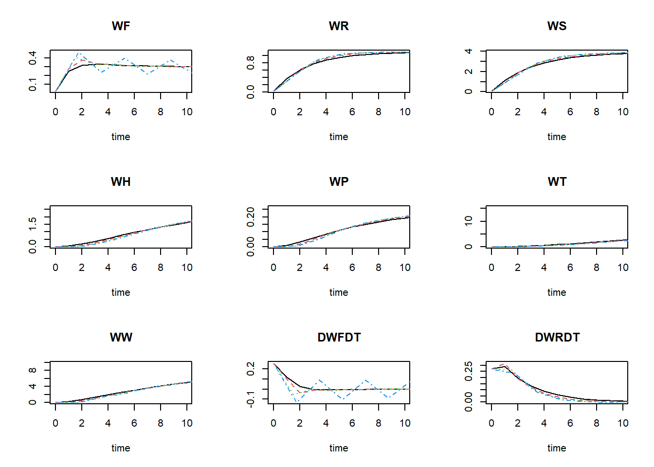
To get the relative difference between the two integration method at time 50 (here as a fraction of the reference ode45, rounded off to 4 digits):
round(100 * tail(states_euler1, 1)[,-1] / tail(states_rk,1)[,-1], 4)## WF WR WS WH WP WT WW DWFDT DWRDT DWSDT DWHDT DWPDT DWTDT DWWDT
## 100.0000 100.0000 100.0000 100.0452 100.0258 100.2455 100.2170 8.3137 10.9683 9.4631 56.6129 56.5673 99.6987 80.1710round(100 * tail(states_euler2, 1)[,-1] / tail(states_rk,1)[,-1], 4)## WF WR WS WH WP WT WW DWFDT DWRDT DWSDT DWHDT DWPDT DWTDT DWWDT
## 100.0000 100.0000 100.0000 100.0582 100.0333 99.6274 100.2754 2364.4260 4.6134 -0.1001 44.1689 44.1292 100.5793 74.8511round(100 * tail(states_euler3, 1)[,-1] / tail(states_rk,1)[,-1], 4)## WF WR WS WH WP WT WW DWFDT DWRDT DWSDT DWHDT
## 8.985990e+01 9.992870e+01 9.994260e+01 1.000613e+02 1.000500e+02 9.892820e+01 1.006107e+02 -6.982504e+08 -5.852244e+05 6.761325e+05 -1.407410e+01
## DWPDT DWTDT DWWDT
## -2.355138e+02 1.014817e+02 -2.811483e+02and here as a relative difference:
round(100 * abs ( (tail(states_euler1, 1)[,-1] - tail(states_rk,1)[,-1]) / tail(states_rk,1)[,-1] ), 4)## WF WR WS WH WP WT WW DWFDT DWRDT DWSDT DWHDT DWPDT DWTDT DWWDT
## 0.0000 0.0000 0.0000 0.0452 0.0258 0.2455 0.2170 91.6863 89.0317 90.5369 43.3871 43.4327 0.3013 19.8290round(100 * abs ( (tail(states_euler2, 1)[,-1] - tail(states_rk,1)[,-1]) / tail(states_rk,1)[,-1] ), 4)## WF WR WS WH WP WT WW DWFDT DWRDT DWSDT DWHDT DWPDT DWTDT DWWDT
## 0.0000 0.0000 0.0000 0.0582 0.0333 0.3726 0.2754 2264.4260 95.3866 100.1001 55.8311 55.8708 0.5793 25.1489round(100 * abs ( (tail(states_euler3, 1)[,-1] - tail(states_rk,1)[,-1]) / tail(states_rk,1)[,-1] ), 4)## WF WR WS WH WP WT WW DWFDT DWRDT DWSDT DWHDT DWPDT
## 1.014010e+01 7.130000e-02 5.740000e-02 6.130000e-02 5.000000e-02 1.071800e+00 6.107000e-01 6.982505e+08 5.853244e+05 6.760325e+05 1.140741e+02 3.355138e+02
## DWTDT DWWDT
## 1.481700e+00 3.811483e+02As you can see in these values, as well as in the figures above: the Euler integration method with smaller time-step better approaches the variable time-step Runge-Kutta method. Using the Euler integration method, when the time-step increases, the deviation from the Runge-Kutta solution increases. Thus, this pattern demonstrates the expected pattern of time-step convergence.
To get the information needed to compute the time coefficients (the
value of the state variables when the system is in equilibrium, but also
the rates of change of the state variables over time), we have to change
AUX <- NULL in function RatesCO2fix to
AUX <- RATES.
##      time        WF        WR        WS         WH         WP         WT        WW        DWFDT      DWRDT     DWSDT      DWHDT      DWPDT      DWTDT
## [1,]    0 0.0200000 0.0200000 0.0600000 0.00000000 0.00000000 0.00000000 0.0000000  0.257495098 0.27349510 0.8234853 0.00600000 0.00120000 0.00480000
## [2,]    1 0.2774951 0.2934951 0.8834853 0.00600000 0.00120000 0.00480000 0.0310000  0.099690951 0.31688703 0.9939354 0.08744853 0.01718971 0.07106282
## [3,]    2 0.3771860 0.6103821 1.8774206 0.09344853 0.01838971 0.07586282 0.4656674 -0.038035918 0.19375410 0.6612510 0.17372479 0.03022253 0.15615228
## [4,]    3 0.3391501 0.8041362 2.5386717 0.26717331 0.04861224 0.23201510 1.1156634 -0.012560376 0.11926390 0.4468464 0.21379117 0.03181078 0.21982730
## [5,]    4 0.3265898 0.9234001 2.9855181 0.48096449 0.08042302 0.45184240 1.7586953 -0.009828462 0.07240023 0.3018813 0.22640713 0.02911814 0.26828176
## [6,]    5 0.3167613 0.9958004 3.2873994 0.70737162 0.10954116 0.72012416 2.3924187 -0.006319573 0.04337774 0.2045037 0.22263419 0.02512484 0.30517920
##          DWWDT
## [1,] 0.0310000
## [2,] 0.4346674
## [3,] 0.6499960
## [4,] 0.6430319
## [5,] 0.6337234
## [6,] 0.6076742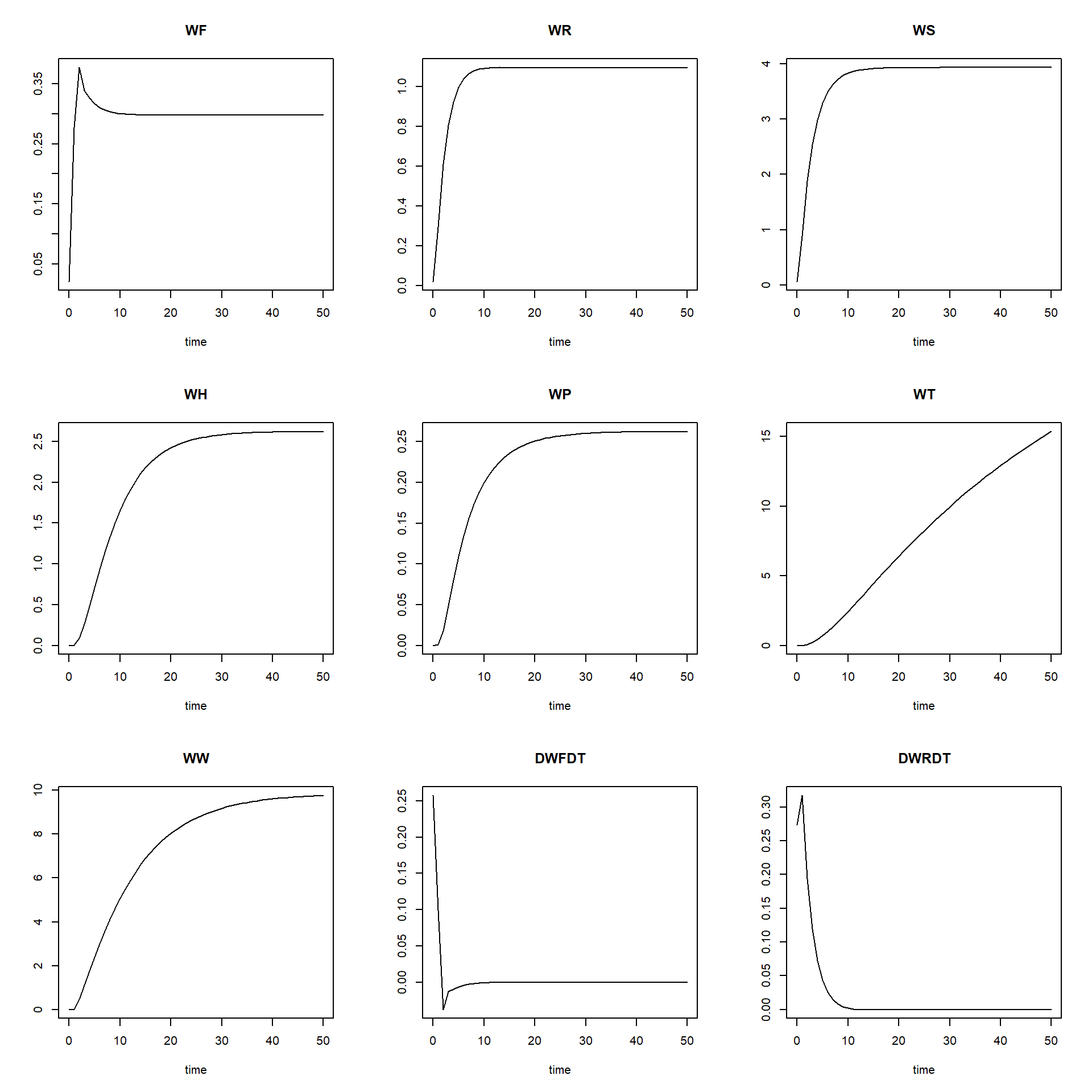
Then, we can define a function that computes the time coefficient; it needs as input a solved model, as well as the time at which the system has reached equilibrium. With this information, we can compute the time coefficients:
tcCO2fix <- function(states, time_equil) {

  # Find index for row with states that are in equilibrium
  ii <- which(states[,"time"] == time_equil)

  # Compute TC for all states using general TC formula
  TC <- data.frame(time = states[,"time"],
                   TC_WF = abs( (states[,"WF"] - states[ii,"WF"]) / states[,"DWFDT"] ),
                   TC_WR = abs( (states[,"WR"] - states[ii,"WR"]) / states[,"DWRDT"] ),
                   TC_WS = abs( (states[,"WS"] - states[ii,"WS"]) / states[,"DWSDT"] ),
                   TC_WP = abs( (states[,"WP"] - states[ii,"WP"]) / states[,"DWPDT"] ))
  return(TC)
}
With a solved model, we can now thus compute the time coefficients, and plot how they vary over time:
states_rk <- ode(y = InitCO2fix(),
                 times = seq(from = 0, to = 50, by = 1),
                 parms = ParmsCO2fix(),
                 func = RatesCO2fix,
                 method = "ode45")
TC <- tcCO2fix(states=states_rk, time_equil = 30)
par(mfrow = c(2,4))
plot(states_rk[,"time"], states_rk[,"WF"], ylab = "WF", xlab = "time", type = "l", col = "black")
plot(states_rk[,"time"], states_rk[,"WR"], ylab = "WR", xlab = "time", type = "l", col = "black")
plot(states_rk[,"time"], states_rk[,"WS"], ylab = "WS", xlab = "time", type = "l", col = "black")
plot(states_rk[,"time"], states_rk[,"WP"], ylab = "WP", xlab = "time", type = "l", col = "black")
plot(TC[,"time"], TC[,"TC_WF"], ylab = "TC WF", xlab = "time", type = "l", col = "black")
plot(TC[,"time"], TC[,"TC_WR"], ylab = "TC WR", xlab = "time", type = "l", col = "black")
plot(TC[,"time"], TC[,"TC_WS"], ylab = "TC WS", xlab = "time", type = "l", col = "black")
plot(TC[,"time"], TC[,"TC_WP"], ylab = "TC WP", xlab = "time", type = "l", col = "black")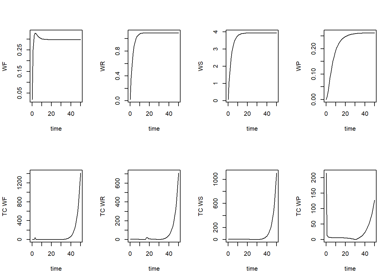
par(mfrow = c(1,1))As we can see, the time coefficients vary quite a bit over time. We may be interested in the minimum time coefficient during times where the system is not yet in equilibrium. Let’s say from the plots that this is up to time 20 We can thus compute the minimum time coefficient up to that time:
TC_sub = subset(TC, time <= 20)
min(TC_sub$TC_WF)
## [1] 0.3755233min(TC_sub$TC_WR)## [1] 0.2652315min(TC_sub$TC_WS)## [1] 3.063995min(TC_sub$TC_WP)## [1] 5.102101Thus, the minimum time coefficient seems to be ca 0.105.
Mass balances tests
To analyse the mass balance of the model, let’s copy-paste the “InitCO2Fix” and “RatesCO2Fix” functions as defined earlier, and add 2 states (IN and OUT), at initial value 0:
InitCO2fix <- function(WF = 0.02, # WF, kgC in Foliage/m2
                       WR = 0.02, # WR, kgC in Roots/m2
                       WS = 0.06, # WS, kgC in Stems/m2
                       WH = 0.0,  # WH, kgC in Stems/m2
                       WP = 0.0,  # WP  kgC in paper/ m2
                       WT = 0.0,  # WT, kgC in timber/m2
                       WW = 0.0   # WW, kgC in waste/m2
                       ){
  # Gather initial conditions in a named vector; given names are names for the state variables in the model
  y <- c(WF = WF,
         WR = WR,
         WS = WS,
         WH = WH,
         WP = WP,
         WT = WT,
         WW = WW,
         IN = 0.0,
         OUT = 0.0)

  # Return
  return(y)
}
In the function computing the rates of change of the state variables with respect to time, we now have to include the rates of change of “IN” and “OUT” as well:
### SAME as earlier, but with specification of mass balance terms MB
RatesCO2fix <- function(t, y, parms) {
  # use the with() function to be able to access the parameters and states easily
  # remember that the with() function is with(data, expr), where
  # - 'data' is ideally a list with named elements
  #   (thus combine 'y' and 'parms' first, using the function c(), then convert to list using as.list())
  # - 'expr' is an expression (i.e. code) that is evaluated
  #   this can span multiple lines of code when embraced with curly brackets {}
  with(
    as.list(c(y, parms)),{

      ### Optional: forcing functions: get value of the driving variables at time t (if any)

      ### Optional: auxiliary equations
      LAI <- WF * SLA / FCL
      IA <- IE *(1 - exp(-K * LAI ))

      PGS <- (1 / (2 * CF)) * (LUE * IA + PC -
                                 sqrt((LUE * IA + PC)^2 -4 * CF * LUE * IA* PC) )
      PG <- PGS * CSPH * CDLH * CDGS * (MWC / (MWC + 2 * MWO))
      PN <- PG - (RF * WF + RR * WR + RS * WS)

      ### Rate equations
      DWFDT <- PN * NF - LRF * WF - NH * WF
      DWRDT <- PN * NR - LRR * WR - NH * WR
      DWSDT <- PN * NS - LRS * WS - NH * WS - TSH*WS
      DWHDT <- TSH* WS - LRS * WH - NH * WH

      HT <- NH * (WF + WR + WS + WH) # total harvest
      HU <- NH * (WS + WH)           # useful harvest

      # The useful harvest, HU, is only the stem, so: (NH*DWS).
      # This is distributed over the two states paper and timber. These are
      # fractions of the useful harvest: paper NP; timber NT=(1-NP).
      DWPDT <- HU * NP - LRP * WP # paper
      DWTDT <- HU * NT - LRT * WT # Timber
      DWWDT <- HT - HU + LRF * WF + LRR * WR +LRS *(WS+WH) - LRW * WW # Waste

      ### Gather all rates of change in a vector
      # - the rates should be in the same order as the states (as specified in 'y')
      # - it can be a named vector, but does not need to be
      RATES <- c(DWFDT = DWFDT,
                 DWRDT = DWRDT,
                 DWSDT = DWSDT,
                 DWHDT = DWHDT,
                 DWPDT = DWPDT,
                 DWTDT = DWTDT,
                 DWWDT = DWWDT)

      ### Optional: get in/out flow used to compute mass balances (or set MB <- NULL)
      RIN  = PN
      ROUT = LRP *WP + LRT * WT + LRW * WW
      MB <- c(IN = RIN, OUT = ROUT)

      ### Optional: gather auxiliary variables that should be returned (or set AUX <- NULL)
      # - this should be a named vector or list!
      AUX <- NULL

      # Return result as a list
      # - the first element is a vector with the rates of change (in the same order as 'y')
      # - all other elements are (optional) extra output, which should be named
      outList <- list(c(RATES, # the rates of change of the state variables (same order as 'y'!)
                        MB),   # the rates of change of the mass balance terms (or NULL)
                      AUX) # optional additional output per time step
      return(outList)
    })
}
Now, we can solve the model with these extra states using:
states <- ode(y = InitCO2fix(),
              times = seq(from = 0, to = 50, by = 1),
              parms = ParmsCO2fix(),
              func = RatesCO2fix,
              method = "euler")
and plot the result:
plot(states)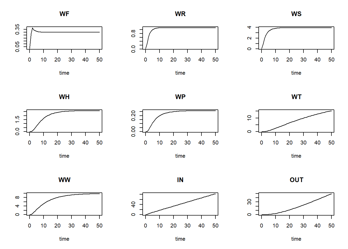
We can now define a function computing the mass balances, one that
needs 2 inputs: state and init, which
respectively are an object as returned by the ode function,
and a vector with initial conditions for the state variables:
MassBalanceCO2fix <- function(y, ini) {
  # Add "0" to the state variables' names to indicate initial condition
  names(ini) = paste0(names(ini), "0")

  # Using the with() function we can access elements directly by there name
  # here: 'y' is a deSolve matrix
  # so it is best to first convert it to a data.frame using function as.data.frame()
  # and then combine it with 'ini' using the function c()
  # and convert to a list using as.list()
  with(as.list(c(as.data.frame(y), ini)), {
    states <- ode(y = InitCO2fix(),
              times = seq(from = 0, to = 50, by = 1),
              parms = ParmsCO2fix(),
              func = RatesCO2fix,
              method = "euler")
    # Compute mass balance terms

    # All that was already  in the system at the start
    INI = sum(ini) # Initial amount of C in the systems, sum of all states, kgC/m2

    # All that is in the system at the end and what left the system
    FIN = y[,"WF"] + y[,"WR"] + y[,"WS"] + y[,"WH"] + y[,"WP"] + y[,"WT"] + y[,"WW"]

    # Balance: difference of all what comes in and goes out
    BAL <- FIN - INI + y[,"OUT"] - y[,"IN"]

    # Return output BAL
    return(BAL)
  })
}
After defining this function, we can check the mass balances per state variable and plot them:
balance <- MassBalanceCO2fix(states, ini = InitCO2fix())
plot(states[,"time"], balance, type = "l", xlab = "time", ylab = "Balance C")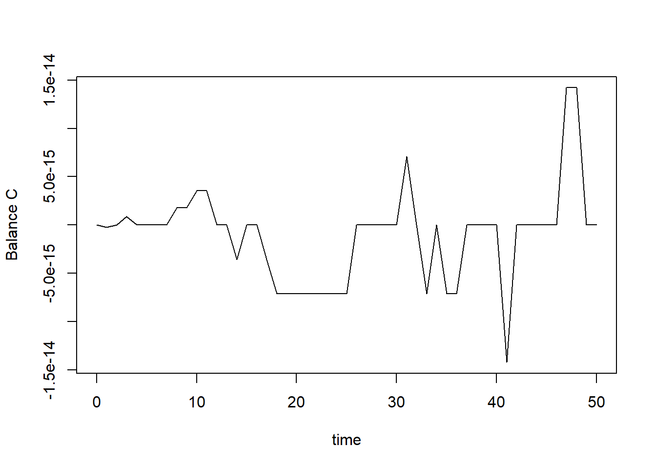
Note that the balances are sufficiently small
(e.g. 1e-14) to consider it effectively zero!