Wageningen University & Research | FEM-31806 | Models for Ecological Systems | FEM | PPS | WEC
Template 2 - Driving variables
This is a code template that you can use as backbone for an R script that implements a model into code in order to solve it numerically, including driving variables and forcing functions.
Code template
A file containing the code template as shown in the code chunk below
can be downloaded
here. Places
indicated by ... need to be filled out (other parts of the
template consist of explanation, and include placeholders for parts that
will be completed in later lectures and templates):
# Template 2 - Driving variables
# See: https://wec.wur.nl/mes for explanation and examples

# Load the deSolve library
library(deSolve)

# Define the forcing function
... <- approxfun(x = ..., y = ..., method = ..., rule = 2)

# Define a function that returns a named vector with initial state values
InitModelname <- function(... = ...) {
  # Gather function arguments in a named vector
  y <- c(... = ...)

  # Return the named vector
  return(y)
}

# Define a function that returns a named vector with parameter values
ParmsModelname <- function(... = ..., # explain the parameter
                           ... = ...  # explain the parameter
                           ) {
  # Gather function arguments in a named vector
  y <- c(... = ...,
         ... = ...)

  # Return the named vector
  return(y)
}

# Define a function for the rates of change of the state variables with respect to time
RatesModelname <- function(t, y, parms) {
  # use the with() function to be able to access the parameters and states easily
  # remember that the with() function is with(data, expr), where
  # - 'data' is ideally a list with named elements
  #   thus: 'y' and 'parms' are combined using function c and converted using function as.list
  # - 'expr' is an expression (i.e. code) that is evaluated
  #   this can span multiple lines of code when embraced with curly brackets {}
  with(
    as.list(c(y, parms)),{

      # Call the forcing functions: get value of the driving variables at time t
      ... <- ...(t)


      # Optional: auxiliary equations
      ...

      # Rate equations
      ...

      # Gather all rates of change in a vector
      # - the rates should be in the same order as the states (as specified in 'y')
      # - it can be a named vector, but does not need to be
      RATES <- c(...)

      # Optional: get in/out flow used to compute mass balances (or set MB <- NULL)
      # see template 4
      MB <- NULL

      # Optional: gather auxiliary variables that should be returned (or set AUX <- NULL)
      # - this should be a named vector or list!
      AUX <- ...

      # Return result as a list
      # - the first element is a vector with the rates of change (in the same order as 'y')
      # - all other elements are (optional) extra output, which should be named
      outList <- list(c(RATES, # the rates of change of the state variables (same order as 'y'!)
                        MB),   # the rates of change of the mass balance terms (or NULL)
                      AUX) # optional additional output per time step
      return(outList)
    }
  )
}

# Define a forcing function that retrieves the value of a driving variable at any point in time
# you may need to load data first
... <- approxfun(x = ..., y = ..., method = ..., rule = 2)

# Numerically solve the model using the ode() function
states <- ode(y = InitModelname(...),
              times = seq(from = ..., to = ..., by = ...),
              func = RatesModelname,
              parms = ParmsModelname(...),
              method = ...)

# Plot
plot(states)
An example with explanation
Let’s continue the model of logistic population growth of population as developed in Template 1 but now assume that the carrying capacity is not constant over time, but a function of some time-varying external driving variable (here let’s consider it to be an amount of resource with , e.g. grass if the population is a grazer species):
where is the carrying capacity, is a driving variable, and two parameters that relate to in a linear fashion. The rate of change of population with respect to time thus becomes:
Because we now we create a new model, let’s call the model Logistic2, and thus names the 3 functions that we need to define: InitLogistic2, ParmsLogistic2 and RatesLogistic2.
Initial state variables
As in Template 1, we define a function that returns a named vector with initial state values:
InitLogistic2 <- function(N = 5) {
  # Gather function arguments in a named vector
  y <- c(N = N)

  # Return the named vector
  return(y)
}
Parameter values
Likewise, we update the function ParmsLogistic defined
in Template 1 to include the 2 new parameters and :
ParmsLogistic2 <- function(r = 0.3, # intrinsic population growth rate
                           k0 = 80, # intercept of the linear relationship between K and x
                           k1 = 2   # slope of the linear relationship between K and x
                           ){
  # Gather function arguments in a named vector
  y <- c(r = r,
         k0 = k0,
         k1 = k1)

  # Return the named vector
  return(y)
}
Driving variables
Sometimes, the modelled dynamical system is dependent on external
driving variables, i.e., variables that are external to the system and
not explicitly modelled (here: grass biomass ). Suppose that we have measurements of
grass biomass at times 0, 1, … 50. If we have the data stored in a file
we can load it into R (e.g. using read.csv for comma
separated files, csv), but now let’s load it into a data.frame called
grassBiomass using:
grassBiomass <- data.frame(time = 0:50,
                           grass = c(8.4,8.2,5.3,6.7,7.4,12.3,15.0,13.6,9.2,10.5,12.0,13.6,14.4,11.7,
                                     12.0,13.6,12.5,9.3,10.8,12.3,11.3,14.9,11.2,11.2,5.1,6.4,10.9,
                                     11.2,9.8,11.5,9.0,10.2,6.5,5.0,6.3,6.6,12.5,15.0,12.1,12.0,12.5,
                                     12.0,12.1,13.9,11.3,9.6,11.5,8.2,9.7,10.1,8.5))
Let’s check the data and plot grass biomass as function of time:
head(grassBiomass)## time grass
## 1 0 8.4
## 2 1 8.2
## 3 2 5.3
## 4 3 6.7
## 5 4 7.4
## 6 5 12.3plot(grassBiomass$time, grassBiomass$grass, pch = 16, xlab = "Time", ylab = "Grass")
lines(grassBiomass$time, grassBiomass$grass, lty = 2)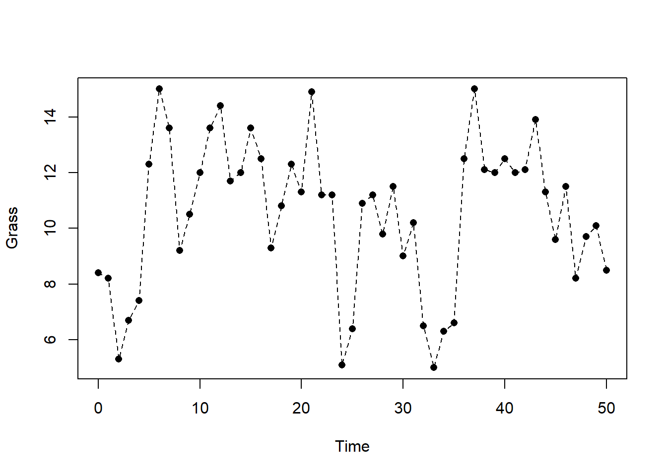
Note that the plotted points give the measured grass biomass as specific points in time, whereas the dashed line connects these points in a linear fashion. Thus, for most of the time we do not have measured values of grass biomass, but when we are certain enough that a linear interpolation between measured values gives a reasonable approximation of grass biomass, then the dashed line (i.e., linear interpolation) approximates the grass biomass at any point in time. However, linear interpolation is not always the preferred choice, and we may opt for non-linear interpolation, or rather want to use the value of the most recent measurement.
Because when solving a model we need the value of the driving
variable (here grass biomass) at any moment in time, we need to
define a forcing function that takes time as input,
and returns the corresponding value of the driving variable. For this,
we can use the approxfun function: a function that takes
x (here time) and y (here
grass) values as inputs, and returns a function that
computes an approximation of the y-variable (here: grass) given the
value of the x-variable (the function’s input argument; here: time).
Check the ?approxfun() help file for documentation.
Here, let’s create 2 forcing functions, one for a linear
interpolation (let’s call it grass_linear), and one for
retrieving the last known value (let’s call it
grass_constant):
grass_linear   <- approxfun(x = grassBiomass$time, y = grassBiomass$grass, method = "linear", rule = 2)
grass_constant <- approxfun(x = grassBiomass$time, y = grassBiomass$grass, method = "constant", rule = 2)
Now, grass_linear and grass_constant are
both a function that require 1 input: the time at which we want
to retrieve the approximation of grass biomass. For example, although we
did not measure grass biomass at time , we can now use the
grass_linear function to linearly interpolate between the
grass biomass measured at and :
grass_linear(4.5)## [1] 9.85which is 9.85 and halfway in between 7.4 (at ) and 12.3 (at )! However, the
grass_constant function should now return the value 7.4
(i.e. the most recently measured value before , thus at ):
grass_constant(4.5)## [1] 7.4We can plot the measured and interpolated (both methods, here with time steps of 0.1 time units) grass biomass over time using:
xseq <- seq(from = 0, to = 50, by = 0.1)
plot(grassBiomass$time, grassBiomass$grass, pch = 16, xlab = "Time", ylab = "Grass")
grass_linear   <- approxfun(x = grassBiomass$time, y = grassBiomass$grass, method = "linear", rule = 2)
grass_constant <- approxfun(x = grassBiomass$time, y = grassBiomass$grass, method = "constant", rule = 2)
lines(xseq, grass_constant(xseq), col = 1, lty = 2)
lines(xseq, grass_linear(xseq), col = 2, lty = 2)
legend(x = "bottomright", title = "method",legend = c("linear","constant"), lty = 2, col = 1:2)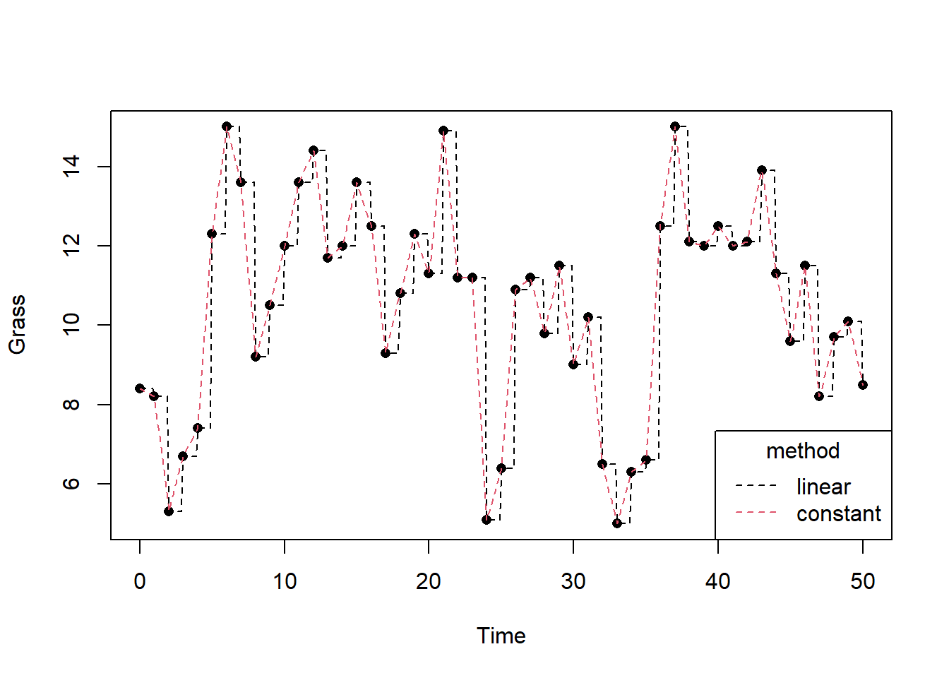
When retrieving the values of driving variables through interpolation, we should always be careful that we do so correctly. In the above example with grass biomass, using either linear or constant interpolation would work, because it is expressed in units without a time dimension. However, when we deal with a driving variable that is for example rainfall in units mm/day, we need to be careful. Suppose that one day has 30 mm of rain, and the next day 0 mm. If we would apply linear interpolation, the values become nonsense values: if we would add the totals up we would get very different values!
Rates of change
Let’s update the RatesLogistic function to include the
driving variable (interpolated in
linear fashion, thus using the grass_linear function), as
well as to compute the value of as
function of , and .
Also, let’s also return the values of
and as additional output:
RatesLogistic2 <- function(t, y, parms) {
  # use the with() function to be able to access the parameters and states easily
  # remember that the with() function is with(data, expr), where
  # - 'data' is ideally a list with named elements
  #   thus: 'y' and 'parms' are combined using function c and converted using function as.list
  # - 'expr' is an expression (i.e. code) that is evaluated
  #   this can span multiple lines of code when embraced with curly brackets {}
  with(
    as.list(c(y, parms)),{

      # Optional: forcing functions: get value of the driving variables at time t (if any)
      x <- grass_linear(t) # here we use linear interpolation between the measured grass biomass values

      # Optional: auxiliary equations
      K <- k0 + k1 * x # Compute carrying capacity K as function of x

      # Rate equations
      dNdt <- r*N*(1-N/K)

      # Gather all rates of change in a vector
      # - the rates should be in the same order as the states (as specified in 'y')
      # - it can be a named vector, but does not need to be
      RATES <- c(dNdt = dNdt)

      # Optional: get in/out flow used to compute mass balances (or set MB <- NULL)
      # see template 4
      MB <- NULL

      # Optional: gather auxiliary variables that should be returned (or set AUX <- NULL)
      # - this should be a named vector or list!
      AUX <- c(RATES, # here we pass the rate of change of N with respect to time back as auxiliary variable
               x = x, # the value of the driving variable at time t (interpolated)
               K = K) # the value of carrying capacity K at time t

      # Return result as a list
      # - the first element is a vector with the rates of change (in the same order as 'y')
      # - all other elements are (optional) extra output, which should be named
      outList <- list(c(RATES, # the rates of change of the state variables
                        MB),   # the rates of change of the mass balance terms if MB is not NULL
                      AUX) # optional additional output per time step
      return(outList)
    }
  )
}
Solving the model
With the functions being defined, we can now solve the model numerically (requesting output for times from 0 to 50 in time steps of 1, using the adaptive stepsize Runge-Kutta integration method “ode45”) and explore the results:
states <- ode(y = InitLogistic2(),
              times = seq(from = 0, to = 50, by = 1),
              func = RatesLogistic2,
              parms = ParmsLogistic2(),
              method = "ode45")
Exploring the solved model
head(states)## time N dNdt x K
## [1,] 0 5.000000 1.422521 8.4 96.8
## [2,] 1 6.629236 1.852007 8.2 96.4
## [3,] 2 8.731539 2.367012 5.3 90.6
## [4,] 3 11.407815 3.004342 6.7 93.4
## [5,] 4 14.772602 3.741180 7.4 94.8
## [6,] 5 18.959700 4.656925 12.3 104.6plot(states)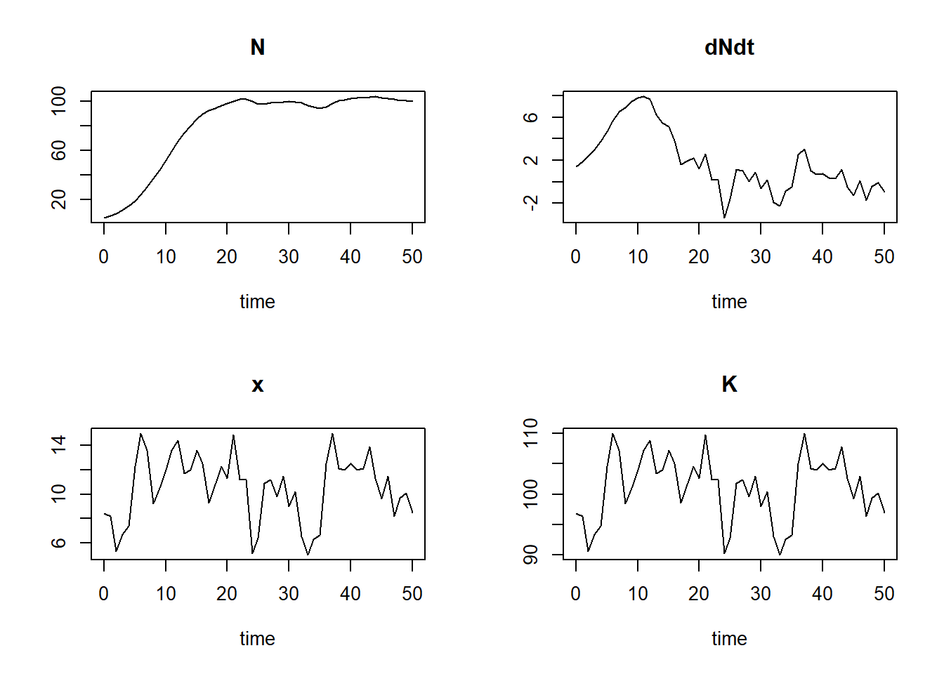
Downloadable R script
An R script with the code chunks of the above example can be downloaded here.