Wageningen University & Research | FEM-31806 | Models for Ecological Systems | FEM | PPS | WEC
NUCOM - Day 3
Aims
Time step convergence
Compare different methods of integration for different time steps. Note that you can simply set these as arguments for your model calling function
ode. Compare the Euler method with a variable time-step 4th order Runga-Kutta method (“ode45”). Run the model with Euler for a time step of 0.1, 1 and 2.5 years. Save the output with computed states for these runs with Euler and save also one output for a run with ode45 as method. For a direct comparison with output at exactly the same moments in time for both integration methods, you can define the variabledeltand adjust the sequence that you use to define the output for time (e.g.:seq(0, 1000, by=delt)). Note that the actual time-steps taken by when using the ode45 integration method will be smaller as the time step is in this method adjusted when required.Plot the state variables of the 4 simulations against time in the same plot. Alternatively, plot the state variables of each of the three Euler simulations with those computed with the ode45 integration method in a plot. Limit the plotting ranges for the x- and y by setting
xlim = c(... , ...)andylim = c(... , ...)to zoom in to times when the model outputs quickly change. What can you roughly conclude for the appropriate time step using Euler?You can also calculate the relative deviation of Euler when compared to the ode45 results (by computing |Euler state-RK state|/RK state , for example at time = 150 years). Within what range of time-step values do state variables not differ more than 1% after a reasonable time period (150 years)?
Develop an equation to calculate the time coefficients for each of the state variables. Implement them and plot time coefficients against time.
Mass balances tests
- Choose the appropriate mass variables in your model, either C, P or N if present.
- Define the sum of all the mass inflows and all the sum of all mass outflows for each of your mass variables in the model.
- Define the balance for each of the mass variables in the model.
- Create a plot to check the mass balance visually: in other words, check the dynamics in each of the mass variables over time. What is your expectation? Is your expectation supported by the graphical output?
Answers
Download here the code as shown on this page in a separate .r file.
Compare integration methods
To check for the difference between Euler and Runge-Kutta
integration, let’s solve the model numerically for 150 time-units in
time-steps of 0.1, 1 and 2.5 (the fixed time-step of the
euler method), as well as with a variable time-step
Runge-Kutta method (ode45, here with output every
time-step):
states_rk <- ode(y = InitNUCOM(),
                 times = seq(from = 1, to = 150, by = 1),
                 parms = ParmsNUCOM(),
                 func = RatesNUCOM,
                 method = "ode45")

delt <- 0.1
states_euler1 <- ode(y = InitNUCOM(),
                     times = seq(from = 1, to = 150, by = delt),
                     parms = ParmsNUCOM(),
                     func = RatesNUCOM,
                     method = "euler")

delt <- 1
states_euler2 <- ode(y = InitNUCOM(),
                     times = seq(from = 1, to = 150, by = delt),
                     parms = ParmsNUCOM(),
                     func = RatesNUCOM,
                     method = "euler")

delt <- 2.5
states_euler3 <- ode(y = InitNUCOM(),
                     times = seq(from = 1, to = 150, by = delt),
                     parms = ParmsNUCOM(),
                     func = RatesNUCOM,
                     method = "euler")
We can have a look at the output of the last time-steps (for all 4 solutions):
tail(states_rk)## time BC1 BC2 BN1 BN2 SC1 SC2 SN1 SN2 DBC1DT DBC2DT DBN1DT DBN2DT DSC1DT DSC2DT
## [145,] 145 33.19373 978.1729 0.6638745 19.56346 533.6164 3632.280 26.07603 129.5436 -0.07003527 0.10582138 -0.0014007053 0.0021164277 -22.77308 8.608356
## [146,] 146 33.13317 978.2643 0.6626635 19.56529 511.7119 3639.973 24.96740 130.0306 -0.05196526 0.07835263 -0.0010393053 0.0015670526 -21.05705 6.844261
## [147,] 147 33.08825 978.3320 0.6617649 19.56664 491.4613 3646.088 23.92360 130.4281 -0.03855604 0.05806538 -0.0007711208 0.0011613076 -19.46396 5.437733
## [148,] 148 33.05491 978.3821 0.6610982 19.56764 472.7454 3650.944 22.94165 130.7515 -0.02860624 0.04305216 -0.0005721249 0.0008610431 -17.98668 4.317387
## [149,] 149 33.03018 978.4194 0.6606036 19.56839 455.4518 3654.799 22.01859 131.0142 -0.02122376 0.03192947 -0.0004244752 0.0006385894 -16.61803 3.425776
## [150,] 150 33.01183 978.4470 0.6602366 19.56894 439.4754 3657.856 21.15150 131.2270 -0.01574633 0.02368401 -0.0003149266 0.0004736801 -15.35094 2.716765
## DSN1DT DSN2DT
## [145,] -1.1420457 0.5377194
## [146,] -1.0757181 0.4394134
## [147,] -1.0123784 0.3580836
## [148,] -0.9520153 0.2910780
## [149,] -0.8945932 0.2360760
## [150,] -0.8400573 0.1910740tail(states_euler1)## time BC1 BC2 BN1 BN2 SC1 SC2 SN1 SN2 DBC1DT DBC2DT DBN1DT DBN2DT DSC1DT DSC2DT
## [1486,] 149.5 33.01525 978.4418 0.6603050 19.56884 445.7793 3657.028 21.51180 131.1651 -0.01676764 0.02521849 -0.0003353528 0.0005043698 -15.85320 2.910913
## [1487,] 149.6 33.01358 978.4443 0.6602715 19.56889 444.1940 3657.319 21.42545 131.1855 -0.01626709 0.02446536 -0.0003253419 0.0004893073 -15.72738 2.843321
## [1488,] 149.7 33.01195 978.4468 0.6602390 19.56894 442.6213 3657.603 21.33965 131.2055 -0.01578149 0.02373474 -0.0003156298 0.0004746949 -15.60253 2.777283
## [1489,] 149.8 33.01037 978.4492 0.6602074 19.56898 441.0610 3657.881 21.25440 131.2251 -0.01531038 0.02302596 -0.0003062076 0.0004605191 -15.47866 2.712765
## [1490,] 149.9 33.00884 978.4515 0.6601768 19.56903 439.5132 3658.152 21.16968 131.2443 -0.01485333 0.02233835 -0.0002970666 0.0004467669 -15.35575 2.649731
## [1491,] 150.0 33.00735 978.4537 0.6601471 19.56907 437.9776 3658.417 21.08549 131.2631 -0.01440993 0.02167128 -0.0002881986 0.0004334257 -15.23379 2.588148
## DSN1DT DSN2DT
## [1486,] -0.8634381 0.2046023
## [1487,] -0.8579945 0.2002562
## [1488,] -0.8525795 0.1959986
## [1489,] -0.8471932 0.1918277
## [1490,] -0.8418353 0.1877420
## [1491,] -0.8365060 0.1837398tail(states_euler2)## time BC1 BC2 BN1 BN2 SC1 SC2 SN1 SN2 DBC1DT DBC2DT DBN1DT DBN2DT DSC1DT DSC2DT
## [145,] 145 33.06542 978.3664 0.6613083 19.56733 515.5680 3644.707 25.37157 130.2503 -0.031742569 0.047732925 -0.0006348514 0.0009546585 -21.40619 5.799998
## [146,] 146 33.03367 978.4141 0.6606735 19.56828 494.1618 3650.507 24.26233 130.6541 -0.022267068 0.033483414 -0.0004453414 0.0006696683 -19.71274 4.450958
## [147,] 147 33.01141 978.4476 0.6602281 19.56895 474.4491 3654.958 23.22083 130.9723 -0.015619919 0.023487617 -0.0003123984 0.0004697523 -18.14908 3.412863
## [148,] 148 32.99579 978.4711 0.6599157 19.56942 456.3000 3658.371 22.24378 131.2224 -0.010956980 0.016475799 -0.0002191396 0.0003295160 -16.70653 2.614915
## [149,] 149 32.98483 978.4876 0.6596966 19.56975 439.5935 3660.986 21.32795 131.4184 -0.007686000 0.011557205 -0.0001537200 0.0002311441 -15.37658 2.002164
## [150,] 150 32.97714 978.4991 0.6595429 19.56998 424.2169 3662.988 20.47016 131.5716 -0.005391482 0.008106965 -0.0001078296 0.0001621393 -14.15106 1.532046
## DSN1DT DSN2DT
## [145,] -1.1092359 0.4037442
## [146,] -1.0415056 0.3182801
## [147,] -0.9770478 0.2501045
## [148,] -0.9158286 0.1959731
## [149,] -0.8577903 0.1531672
## [150,] -0.8028566 0.1194381tail(states_euler3)## time BC1 BC2 BN1 BN2 SC1 SC2 SN1 SN2 DBC1DT DBC2DT DBN1DT DBN2DT DSC1DT DSC2DT
## [55,] 136.0 15.23022 18.09922 0.3046044 0.3619845 383.7939 4691.925 11.96006 137.8455 137.949839 418.11046 2.7589968 8.3622093 -21.56538 -1109.7728
## [56,] 138.5 360.10482 1063.37538 7.2020964 21.2675077 329.8804 1917.493 11.34592 105.6547 -130.170409 -274.71529 -2.6034082 -5.4943058 189.67245 496.8394
## [57,] 141.0 34.67880 376.58716 0.6935759 7.5317431 804.0616 3159.592 20.96198 103.0280 14.489343 332.14137 0.2897869 6.6428274 -43.51765 -419.3736
## [58,] 143.5 70.90215 1206.94058 1.4180431 24.1388117 695.2675 2111.158 20.78216 90.0973 -15.895546 -271.05186 -0.3179109 -5.4210371 -13.08010 579.5686
## [59,] 146.0 31.16329 529.31094 0.6232658 10.5862188 662.5672 3560.079 21.19002 108.5040 7.982520 193.97165 0.1596504 3.8794330 -34.30740 -378.0392
## [60,] 148.5 51.11959 1014.24007 1.0223918 20.2848014 576.7987 2614.981 20.14025 104.3462 -6.276731 -46.00113 -0.1255346 -0.9200226 -15.47214 285.2205
## DSN1DT DSN2DT
## [55,] -0.24565508 -12.876309
## [56,] 3.84642697 -1.050698
## [57,] -0.07192976 -5.172271
## [58,] 0.16314473 7.362689
## [59,] -0.41990835 -1.663132
## [60,] -0.24699267 2.642353Now, you can plot all solutions together in a single figure using:
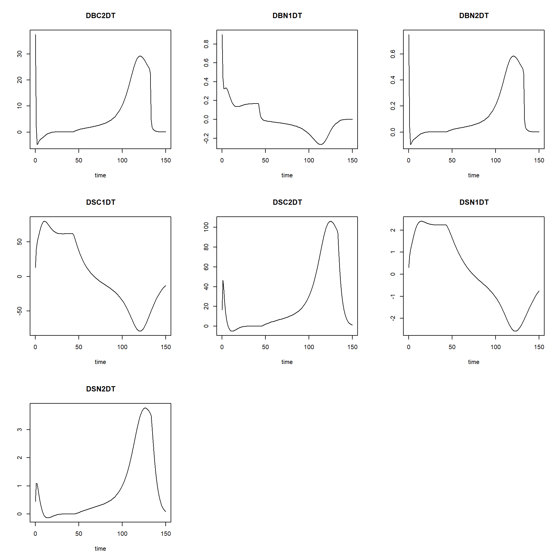
plot(states_rk, states_euler1,states_euler2, states_euler3)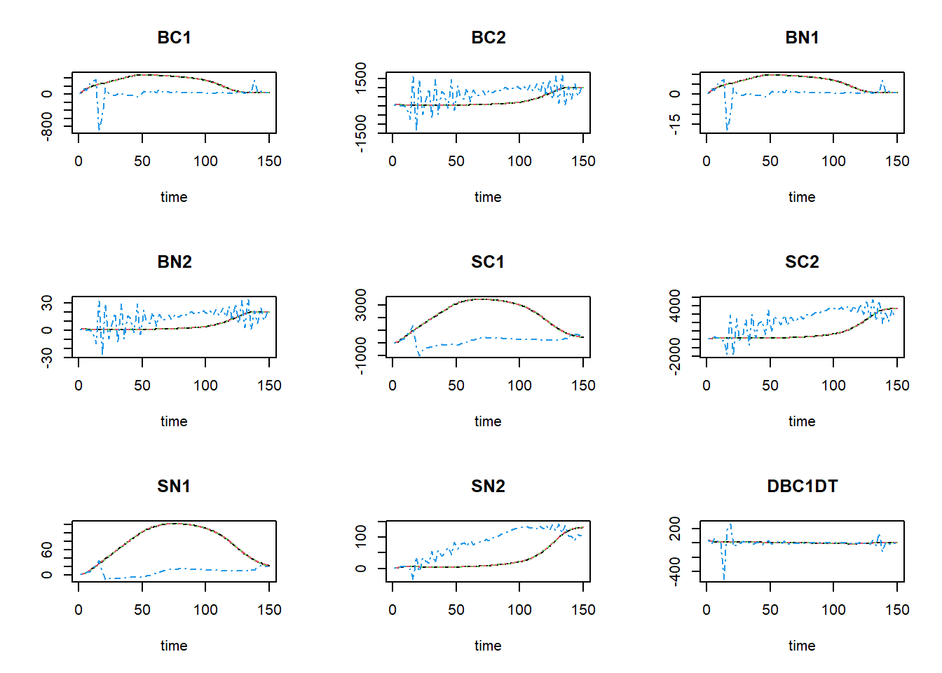
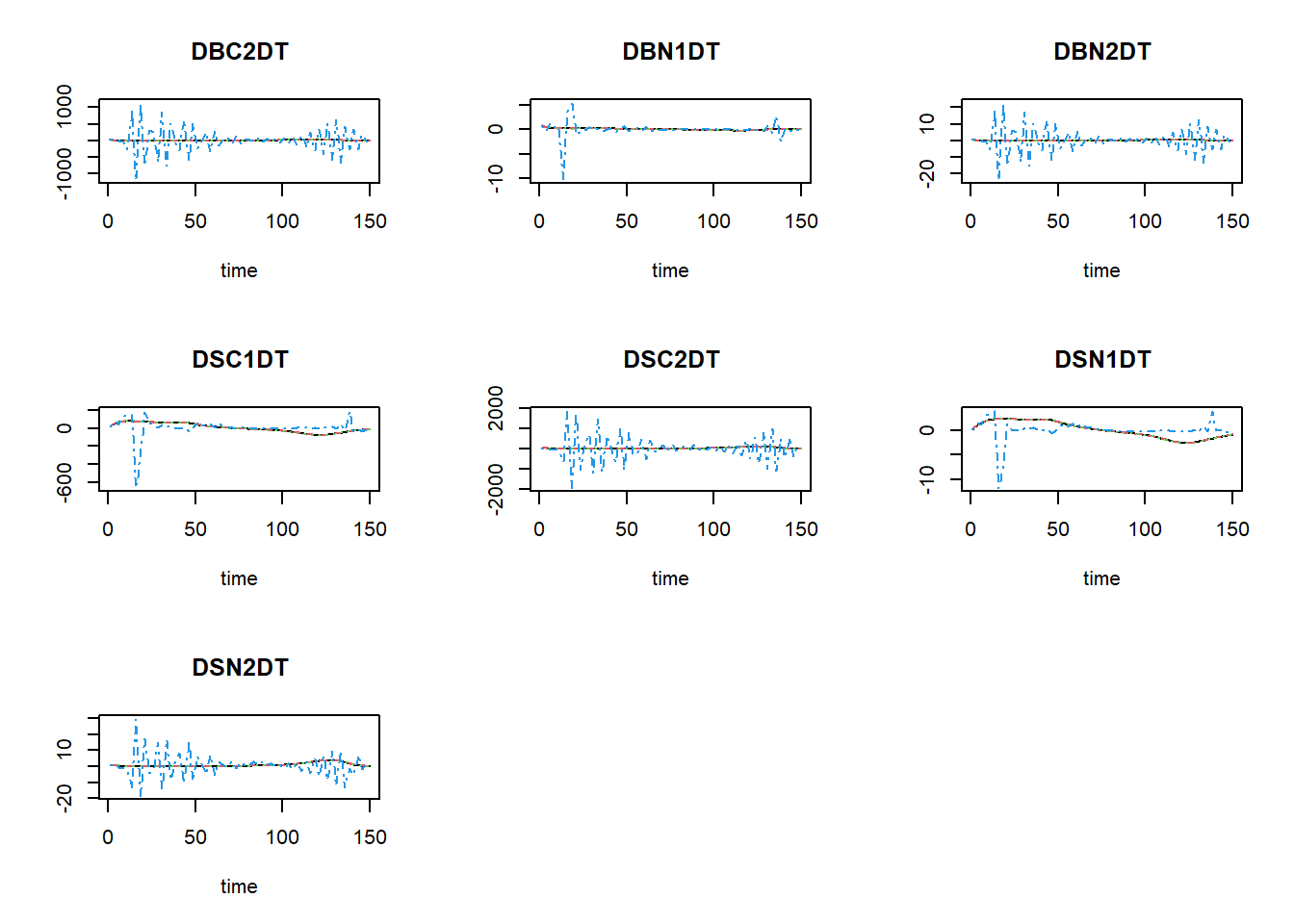
The black line now is the Runge-Kutta solution (with variable
time-step), the dashed red line is the first Euler solution (with
time-step of 0.1), the dashed green line is the second Euler solution
(with time-step of 1), and the dashed blue line is the third Euler
solution (with time-step of 2.5). To focus a bit more on the first time
steps, we can limit the x-axis to a range between 0 and 15 using the
xlim argument:
plot(states_rk, states_euler1,states_euler2, states_euler3, xlim=c(0,15))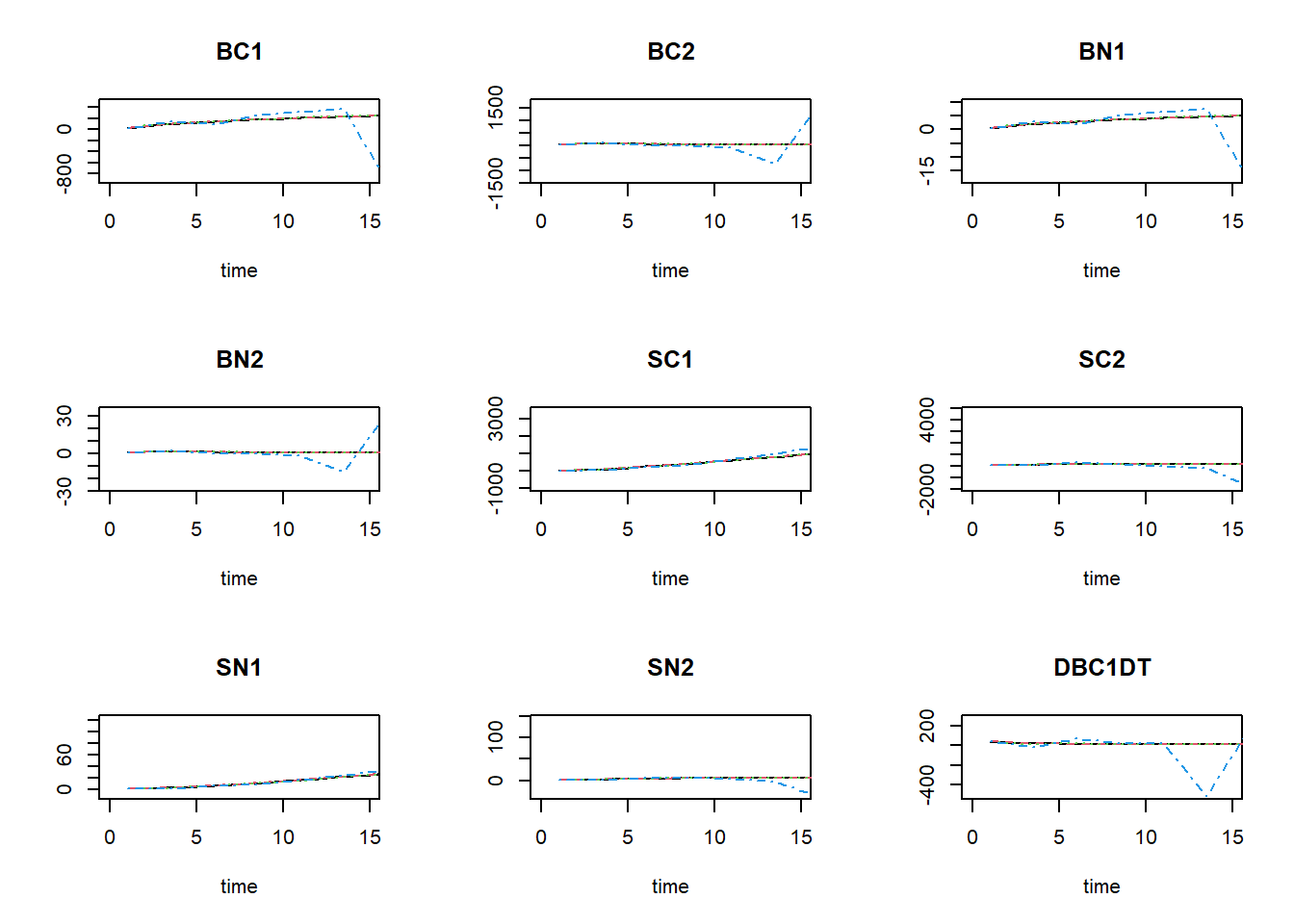
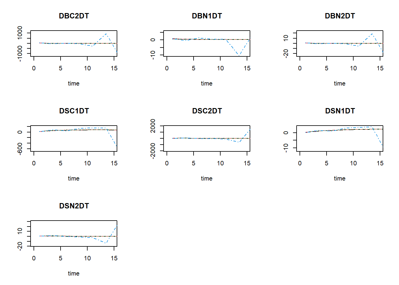
We see that especially for BC1 and BN1 there the solution for Euler with a time-step of 2.5 is quite some difference from the other solutions!
To get the relative difference between the two integration method at time 150 (here as a fraction of the reference ode45, rounded off to 4 digits):
round(100 * tail(states_euler1, 1)[,-1] / tail(states_rk,1)[,-1], 4)## BC1 BC2 BN1 BN2 SC1 SC2 SN1 SN2 DBC1DT DBC2DT DBN1DT DBN2DT DSC1DT DSC2DT DSN1DT DSN2DT
## 99.9864 100.0007 99.9864 100.0007 99.6592 100.0153 99.6879 100.0275 91.5129 91.5018 91.5129 91.5018 99.2369 95.2658 99.5773 96.1616round(100 * tail(states_euler2, 1)[,-1] / tail(states_rk,1)[,-1], 4)## BC1 BC2 BN1 BN2 SC1 SC2 SN1 SN2 DBC1DT DBC2DT DBN1DT DBN2DT DSC1DT DSC2DT DSN1DT DSN2DT
## 99.8949 100.0053 99.8949 100.0053 96.5280 100.1403 96.7788 100.2626 34.2396 34.2297 34.2396 34.2297 92.1837 56.3923 95.5717 62.5088round(100 * tail(states_euler3, 1)[,-1] / tail(states_rk,1)[,-1], 4)## BC1 BC2 BN1 BN2 SC1 SC2 SN1 SN2 DBC1DT DBC2DT DBN1DT DBN2DT
## 154.8523 103.6582 154.8523 103.6582 131.2471 71.4895 95.2190 79.5158 39861.5415 -194228.6694 39861.5415 -194228.6698
## DSC1DT DSC2DT DSN1DT DSN2DT
## 100.7896 10498.5351 29.4019 1382.8953and here as a relative difference:
round(100 * abs ( (tail(states_euler1, 1)[,-1] - tail(states_rk,1)[,-1]) / tail(states_rk,1)[,-1] ), 4)## BC1 BC2 BN1 BN2 SC1 SC2 SN1 SN2 DBC1DT DBC2DT DBN1DT DBN2DT DSC1DT DSC2DT DSN1DT DSN2DT
## 0.0136 0.0007 0.0136 0.0007 0.3408 0.0153 0.3121 0.0275 8.4871 8.4982 8.4871 8.4982 0.7631 4.7342 0.4227 3.8384round(100 * abs ( (tail(states_euler2, 1)[,-1] - tail(states_rk,1)[,-1]) / tail(states_rk,1)[,-1] ), 4)## BC1 BC2 BN1 BN2 SC1 SC2 SN1 SN2 DBC1DT DBC2DT DBN1DT DBN2DT DSC1DT DSC2DT DSN1DT DSN2DT
## 0.1051 0.0053 0.1051 0.0053 3.4720 0.1403 3.2212 0.2626 65.7604 65.7703 65.7604 65.7703 7.8163 43.6077 4.4283 37.4912round(100 * abs ( (tail(states_euler3, 1)[,-1] - tail(states_rk,1)[,-1]) / tail(states_rk,1)[,-1] ), 4)## BC1 BC2 BN1 BN2 SC1 SC2 SN1 SN2 DBC1DT DBC2DT DBN1DT DBN2DT DSC1DT
## 54.8523 3.6582 54.8523 3.6582 31.2471 28.5105 4.7810 20.4842 39761.5415 194328.6694 39761.5415 194328.6698 0.7896
## DSC2DT DSN1DT DSN2DT
## 10398.5351 70.5981 1282.8953As you can see in these values, as well as in the figures above: the Euler integration method with smaller time-step better approaches the variable time-step Runge-Kutta method. At time 150, the state SN1 shows the largest effect of the time-step used in the Euler integration. Using the Euler integration method, when the time-step increases, the deviation from the Runge-Kutta solution increases. Thus, this pattern demonstrates the expected pattern of time-step convergence.
To get the information needed to compute the time coefficients (the
value of the state variables when the system is in equilibrium, but also
the rates of change of the state variables over time), we have to change
AUX <- NULL in function RatesNUCOM to
AUX <- RATES.
##      time       BC1      BC2      BN1      BN2      SC1      SC2      SN1      SN2   DBC1DT    DBC2DT    DBN1DT      DBN2DT   DSC1DT    DSC2DT   DSN1DT
## [1,]    0  25.00000 25.00000 0.500000 0.500000  25.0000  25.0000 0.500000 0.500000 45.00000 37.500000 0.9000000  0.75000000 13.00000 16.500000 0.300000
## [2,]    1  70.00000 62.50000 1.400000 1.250000  38.0000  41.5000 0.800000 0.950000 21.88679  1.863208 0.4377358  0.03726415 38.96000 46.290000 0.836000
## [3,]    2  91.88679 64.36321 1.837736 1.287264  76.9600  87.7900 1.636000 2.039000 16.45824 -4.785207 0.3291649 -0.09570414 48.97528 36.857287 1.092962
## [4,]    3 108.34504 59.57800 2.166901 1.191560 125.9353 124.6473 2.728962 3.112578 16.18878 -4.470243 0.3237756 -0.08940486 54.93220 23.704852 1.279115
## [5,]    4 124.53382 55.10776 2.490676 1.102155 180.8675 148.3521 4.008076 3.999092 16.68932 -3.572219 0.3337864 -0.07144439 60.25089 13.992468 1.455333
## [6,]    5 141.22314 51.53554 2.824463 1.030711 241.1184 162.3446 5.463409 4.681417 16.64351 -3.036294 0.3328702 -0.06072588 65.44441  7.419279 1.630573
##         DSN2DT
## [1,] 0.4500000
## [2,] 1.0890000
## [3,] 1.0735777
## [4,] 0.8865144
## [5,] 0.6823248
## [6,] 0.4972822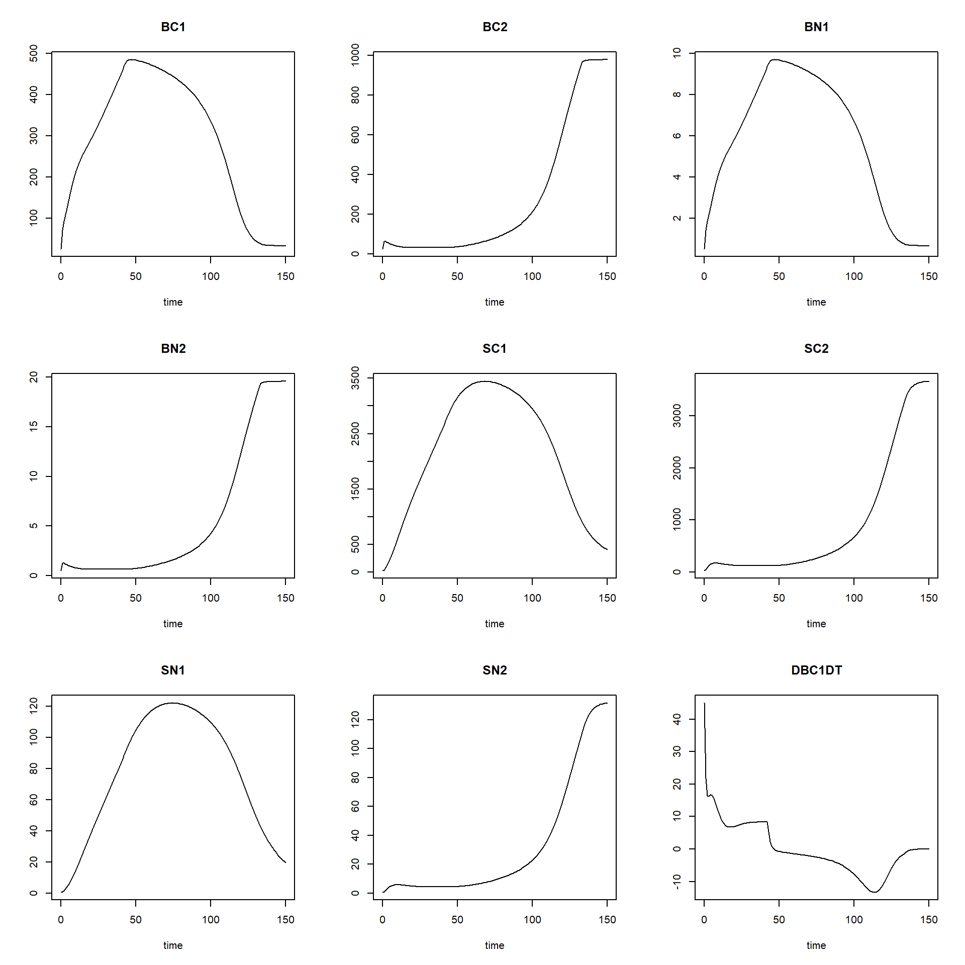
Then, we can define a function that computes the time coefficient; it needs as input a solved model, as well as the time at which the system has reached equilibrium. With this information, we can compute the time coefficients:
tcNUCOM <- function(states, time_equil){

  # Find index for row with states that are in equilibrium
  ii <- which(states[,"time"] == time_equil)

  # Compute TC for all states using general TC formula
  TC <- data.frame(time = states[,"time"],
                   TC_BC1 = abs( (states[,"BC1"] - states[ii,"BC1"]) / states[,"DBC1DT"] ),
                   TC_BC2 = abs( (states[,"BC2"] - states[ii,"BC2"]) / states[,"DBC2DT"] ),
                   TC_BN1 = abs( (states[,"BN1"] - states[ii,"BN1"]) / states[,"DBN1DT"] ),
                   TC_BN2 = abs( (states[,"BN2"] - states[ii,"BN2"]) / states[,"DBN2DT"] ),
                   TC_SC1 = abs( (states[,"SC1"] - states[ii,"SC1"]) / states[,"DSC1DT"] ),
                   TC_SC2 = abs( (states[,"SC2"] - states[ii,"SC2"]) / states[,"DSC2DT"] ),
                   TC_SN1 = abs( (states[,"SN1"] - states[ii,"SN1"]) / states[,"DSN1DT"] ),
                   TC_SN2 = abs( (states[,"SN2"] - states[ii,"SN2"]) / states[,"DSN2DT"] ))
  return(TC)
}
With a solved model, we can now thus compute the time coefficients, and plot how they vary over time:
states <- ode(y = InitNUCOM(),
              times = seq(from = 1, to = 150, by = 1),
              parms = ParmsNUCOM(),
              func = RatesNUCOM,
              method = "ode45")
TC <- tcNUCOM(states = states, time_equil = 150)
par(mfrow = c(2,2))
ymax <- max(max(states[,"BC1"]), max(states[,"BC2"]),
max(states[,"SC1"]), max(states[,"SC2"]))
plot(states[,"time"], states[,"BC1"], type = "l", ylim = c(0,ymax),
col = "black", xlab = "time", ylab = "Carbon, gC/m2")
lines(states[,"time"], states[,"BC2"], col = "grey")
lines(states[,"time"], states[,"SC1"], col = "red")
lines(states[,"time"], states[,"SC2"], col = "orange")
ymax <- max(max(states[,"BN1"]), max(states[,"BN2"]),
max(states[,"SN1"]), max(states[,"SN2"]))
plot(states[,"time"], states[,"BN1"], type = "l", ylim = c(0,ymax),
col="black", xlab = "time", ylab = "Nitrogen, gN/m2")
lines(states[,"time"], states[,"BN2"], col = "grey")
lines(states[,"time"], states[,"SN1"], col = "red")
lines(states[,"time"], states[,"SN2"], col = "orange")
ymax <- max(max(TC[,"TC_BC1"]), max(TC[,"TC_BC2"]),
max(TC[,"TC_SC1"]), max(TC[,"TC_SC2"]))
plot(TC[,"time"], TC[,"TC_BC1"], type = "l", ylim = c(0,ymax),
col = "black", xlab = "time", ylab = "TC")
lines(TC[,"time"], TC[,"TC_BC2"], col = "grey")
lines(TC[,"time"], TC[,"TC_SC1"], col = "red")
lines(TC[,"time"], TC[,"TC_SC2"], col = "orange")
ymax <- max(max(TC[,"TC_BN1"]), max(TC[,"TC_BN2"]),
max(TC[,"TC_SN1"]), max(TC[,"TC_SN2"]))
plot(TC[,"time"], TC[,"TC_BN1"], type = "l", ylim = c(0,ymax),
col="black", xlab = "time", ylab = "TC")
lines(TC[,"time"], TC[,"TC_BN2"], col = "grey")
lines(TC[,"time"], TC[,"TC_SN1"], col = "red")
lines(TC[,"time"], TC[,"TC_SN2"], col = "orange")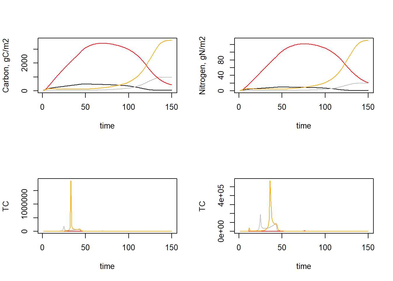
par(mfrow = c(1,1))As we can see, the time coefficients vary quite a bit over time. We may be interested in the minimum time coefficient during times where the system is not yet in equilibrium. Let’s say from the plots that this is up to time 100 We can thus compute the minimum time coefficient up to that time:
TC_sub = subset(TC, time <= 100)
min(TC_sub[,-1])
## [1] 0.1780407Thus, the minimum time coefficient seems to be ca 0.177.
Mass balances tests
To analyse the mass balance of the model, let’s copy-paste the “InitNUCOM” and “RatesNUCOM” functions as defined earlier, and add 4 extra states (IN and OUT, both for C and for N), at initial value 0:
InitNUCOM <- function(
  # For the vegetation
  BC1 = 25.0,  # gC in Veg.1 / m2
  BC2 = 25.0,  # gC in Veg.2 / m2
  BN1 = 0.5,   # gN in Veg.1 / m2
  BN2 = 0.5,   # gN in Veg.2 / m2

  # For the soil
  SC1 = 25.0, # gC from Veg.1 / m2
  SC2 = 25.0, # gC from Veg.2 / m2
  SN1 = 0.5,  # gN from Veg.1 / m2
  SN2 = 0.5   # gN from Veg.2 / m2
  ) {
  # Gather initial conditions in a named vector; given names are names for the state variables in the model
  y <- c(BC1 = BC1, BC2 = BC2,
         BN1 = BN1, BN2 = BN2,
         SC1 = SC1, SC2 = SC2,
         SN1 = SN1, SN2 = SN2,
         CIN = 0.0, COUT = 0.0, # mass balance terms for C
         NIN = 0.0, NOUT = 0.0) # mass balance terms for N

  # Return
  return(y)
}
In the function computing the rates of change of the state variables with respect to time, we now have to include the rates of change of “IN” and “OUT” (for both C and N) as well:
RatesNUCOM <- function(t, y, parms) {
  # use the with() function to be able to access the parameters and states easily
  # remember that the with() function is with(data, expr), where
  # - 'data' is ideally a list with named elements
  #   thus: 'y' and 'parms' are combined using function c and converted using function as.list
  # - 'expr' is an expression (i.e. code) that is evaluated
  #   this can span multiple lines of code when embraced with curly brackets {}
  with(
    as.list(c(y, parms)),{

      ### Optional: forcing functions: get value of the driving variables at time t (if any)

      ### Optional: auxiliary equations

      # Litter production of both species in terms of Carbon and Nitrogen
      LITPC1 <- BC1 * MORT1
      LITPC2 <- BC2 * MORT2
      LITPN1 <- BN1 * MORT1
      LITPN2 <- BN2 * MORT2

      # Decomposition of soil organic matter in terms of carbon and nitrogen
      # DECOM is the net carbon production, lost as CO2-C from the system
      DECOM1 <- SC1 * DECAY1 * (1.0 - EFFMO)
      DECOM2 <- SC2 * DECAY2 * (1.0 - EFFMO)

      # Definition of details of overall input-output rate equations
      # Mineralisation of Nitrogen
      MINER1 <- DECAY1 * SC1*( (SN1/SC1) - (NCONMO/CCONMO)*EFFMO )
      MINER2 <- DECAY2 * SC2*( (SN2/SC2) - (NCONMO/CCONMO)*EFFMO )
      MINTOT <- MINER1 + MINER2

      # Nitrogen supply to (N-deposition) the system
      NDEP <- NDEPCO
      NAVAIL <- NDEP + MINER1 + MINER2

      # Growth rates of both species
      NLIMG1 <- ( BC1/(BC1 + BC2) ) * NAVAIL/NCONC1
      LLIMG1 <- ( BC1/(BC1 + BC2) ) * GMAX1
      ACTGC1 <- pmin(NLIMG1 , LLIMG1)

      NLIMG2 <- ( BC2/(BC1 + BC2) ) * NAVAIL/NCONC2
      LLIMG2 <- ( BC2/(BC1 + BC2) ) * GMAX2
      ACTGC2 <- pmin(NLIMG2 , LLIMG2)

      # Therefore, CO2 evolution is calculated per species and in total as:
      CO21DT <- DECOM1
      CO22DT <- DECOM2
      # TOTCO2 = CO21 + CO22

      # Nitrogen uptake rates of both species
      NUPT1 <- ACTGC1 * NCONC1
      NUPT2 <- ACTGC2 * NCONC2

      # Nitrogen loss (Leaching) from the system
      LEACH <- NAVAIL - NUPT1 - NUPT2

      ### Rate equations
      DBC1DT <- ACTGC1 - LITPC1 + SEEDC1
      DBC2DT <- ACTGC2 - LITPC2 + SEEDC2
      DBN1DT <- NUPT1 - LITPN1 + SEEDN1
      DBN2DT <- NUPT2 - LITPN2 + SEEDN2
      DSC1DT <- LITPC1 - DECOM1
      DSC2DT <- LITPC2 - DECOM2
      DSN1DT <- LITPN1 - MINER1
      DSN2DT <- LITPN2 - MINER2

      ### Gather all rates of change in a vector
      # - the rates should be in the same order as the states (as specified in 'y')
      # - it can be a named vector, but does not need to be
      RATES <- c(DBC1DT = DBC1DT,
                 DBC2DT = DBC2DT,
                 DBN1DT = DBN1DT,
                 DBN2DT = DBN2DT,
                 DSC1DT = DSC1DT,
                 DSC2DT = DSC2DT,
                 DSN1DT = DSN1DT,
                 DSN2DT = DSN2DT)

      ### Optional: get in/out flow used to compute mass balances (or set MB <- NULL)

      # Sum of all outflows: RCOUT = LITPC1+LITPC2 + DECOM1+DECOM2
      DCOUTDT = LITPC1 + LITPC2 + DECOM1 + DECOM2
      # Sum of all inflows: RCIN = ACTGC1+ACTGC2 + SEEDC1+SEEDC2 + LITPC1+LITPC2
      DCINDT = ACTGC1 + ACTGC2 + SEEDC1 + SEEDC2 + LITPC1 + LITPC2

      # Sum of all inflows: RNIN = NUPT1+NUPT2 + SEEDN1+SEEDN2 + LITPN1+LITPN2 + NDEP +  MINER1+MINER2
      DNINDT = NUPT1 + NUPT2 + SEEDN1+ SEEDN2 + LITPN1 + LITPN2 + NDEP +  MINER1 + MINER2

      # Sum of all outflows: RNOUT = LITPN1+LITPN2 + MINER1+MINER2 + LEACH + NUPT1+NUPT2
      DNOUTDT = LITPN1 + LITPN2 + MINER1 + MINER2 + LEACH + NUPT1 + NUPT2

      # To calculate the C-balance (this approach should yield 0.000):
      DCBALDT = (DBC1DT + DBC2DT + DSC1DT + DSC2DT) + DCOUTDT - DCINDT

      # To calculate the N-balance (this approach should yield 0.000):
      DNBALDT = (DBN1DT + DBN2DT + DSN1DT + DSN2DT) + DNOUTDT - DNINDT

      # Combine in a named vector
      MB <- c(DCINDT = DCINDT, DCOUTDT = DCOUTDT,
              DNINDT = DNINDT, DNOUTDT = DNOUTDT)

      ### Optional: gather auxiliary variables that should be returned (or set AUX <- NULL)
      # - this should be a named vector or list!
      AUX <- NULL

      # Return result as a list
      # - the first element is a vector with the rates of change (in the same order as 'y')
      # - all other elements are (optional) extra output, which should be named
      outList <- list(c(RATES, # the rates of change of the state variables (same order as 'y'!)
                        MB),   # the rates of change of the mass balance terms (or NULL)
                      AUX) # optional additional output per time step
      return(outList)
    })
}
Now, we can solve the model with these extra states using:
states <- ode(y = InitNUCOM(),
              times = seq(1, 150, by = 1),
              parms = ParmsNUCOM(),
              func = RatesNUCOM,
              method = "euler")
and plot the result:
plot(states)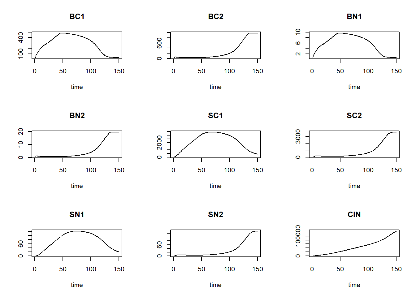
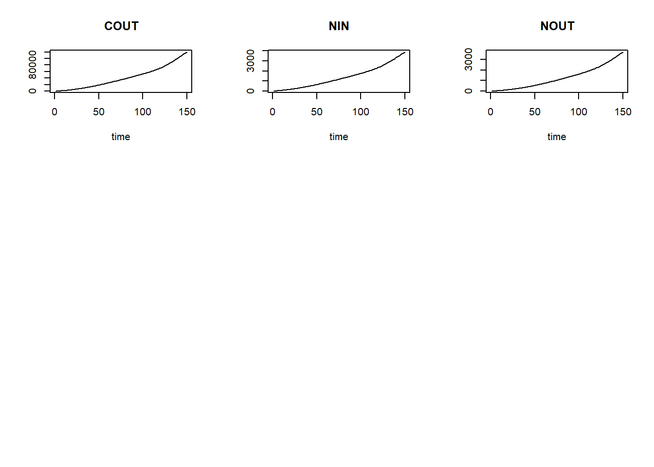
We can now define a function computing the mass balances, one that
needs 2 inputs: state and init, which
respectively are an object as returned by the ode function,
and a vector with initial conditions for the state variables:
MassBalanceNUCOM <- function(y, ini) {
  # Using the with() function we can access elements directly by there name
  # here: 'y' is a deSolve matrix
  # so it is best to first convert it to a data.frame using function as.data.frame()
  # and then combine it with 'ini' using the function c()
  # and convert to a list using as.list()
  with(as.list(c(as.data.frame(y), ini)), {

    # Compute mass balance terms

    # All that was already  in the system at the start
    CINI = ini[["BC1"]] + ini[["BC2"]] + ini[["SC1"]] + ini[["SC2"]] + ini[["CIN"]] + ini[["COUT"]]
    NINI = ini[["BN1"]] + ini[["BN2"]] + ini[["SN1"]] + ini[["SN2"]] + ini[["NIN"]] + ini[["NOUT"]]
    # note: if a "0" is added to the names of 'ini' (as per the template), then here also add "0"!

    # All that is in the system at the end
    CFIN = (y[,"BC1"] + y[,"BC2"] + y[,"SC1"] + y[,"SC2"])
    NFIN = (y[,"BN1"] + y[,"BN2"] + y[,"SN1"] + y[,"SN2"])

    # To calculate the C-balance (this approach should yield 0.000):
    BAL = data.frame(time = y[,"time"],
                     CBAL = CFIN - CINI + y[,"COUT"] - y[,"CIN"],
                     NBAL = NFIN - NINI + y[,"NOUT"] - y[,"NIN"])

    # Return output BAL
    return(BAL)
  })
}
After defining this function, we can check the mass balances per state variable and plot them:
balance = MassBalanceNUCOM(states, ini=InitNUCOM())
par(mfrow = c(2,1))
plot(balance[,"time"], balance[,"CBAL"], type="l", xlab="time", ylab="Balance C")
plot(balance[,"time"], balance[,"NBAL"], type="l", xlab="time", ylab="Balance N")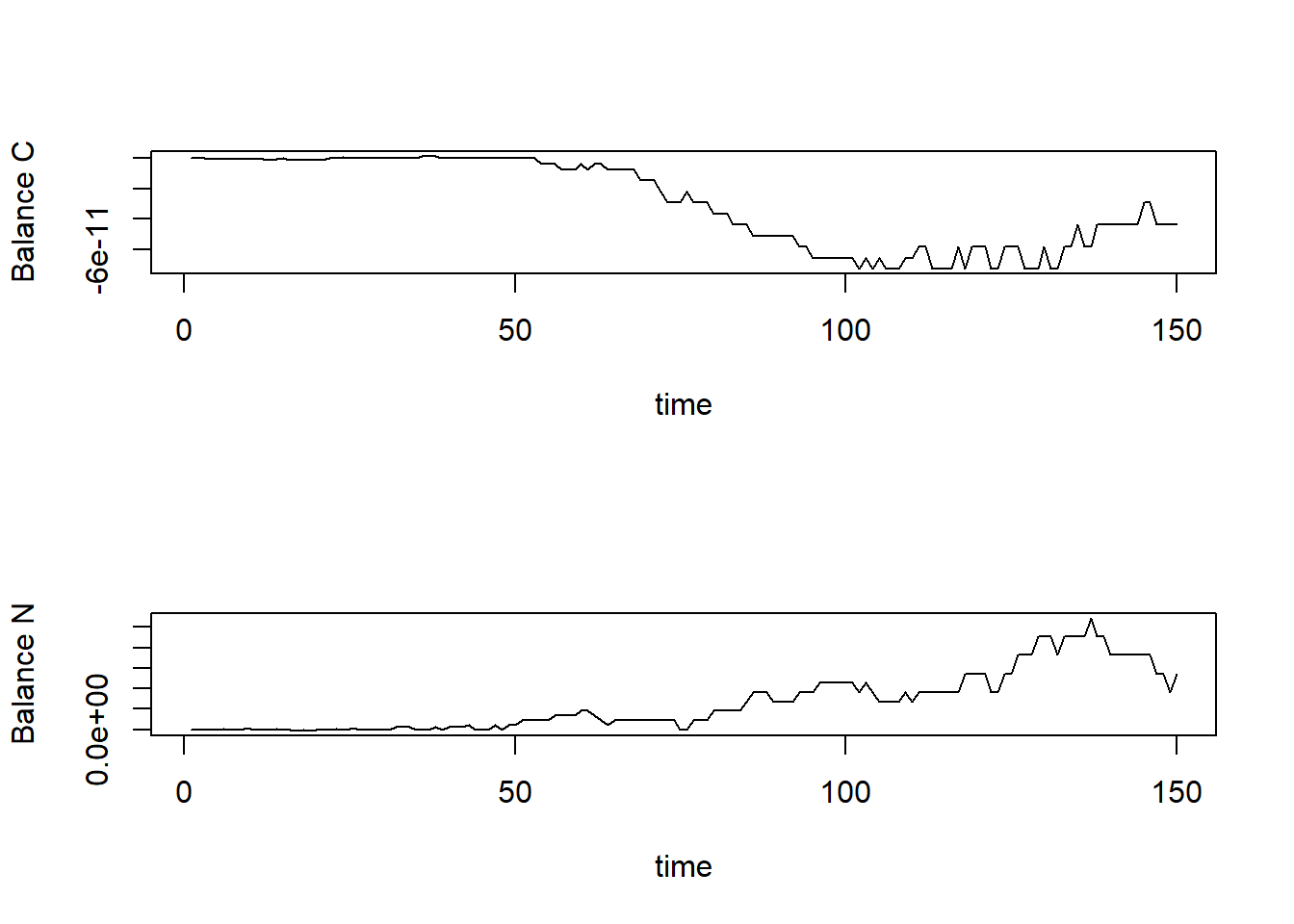
par(mfrow = c(1,1))Note that the balances are sufficiently small
(e.g. 1e-14) to consider it effectively zero!