Wageningen University & Research | FEM-31806 | Models for Ecological Systems | FEM | PPS | WEC
Chapter 7 - Sensitivity analysis
Knowledge questions
Sensitivity analysis plays a central role when working with ODE models. It is not just an optional extra step, it is a key step in figuring out whether your model is trustworthy, how it behaves, and where you can best focus your effort in improving parameter estimates.
Sensitivity analysis reveals which parameter(s) strongly influence model output: high‑sensitivity parameters are parameter where a small change in parameter values causes a big change in modelled response or output state (a state variables of interest). Low‑sensitivity parameters, on the other hand, can be changed without much consequential change in model output; the model is robust to uncertainty in them. Knowing the sensitivity of the model to variation in parameter values is thus very helpful: it helps you avoid wasting much time on estimating parameter values that barely affect the system. Parameters that do not influence model outcomes are even candidates for removal from the model by simplifying the model. If a parameter has almost no influence on the output, its inclusion in the model leads (possibly) to unnessesary complexity. Also, such parameters cannot be reliably estimated from data.
Let be the state variable of interest, thus the model’s outcome, and the parameter of interest, both with their own units, then the Sensitivity Index (SI) is the index that computes the change in when we change the parameter by 1 unit. Thus, the units are . Thus, you can interpret this as “how much does change per unit change in ”.
The SI thus always carries units!
The Elasticity Index (EI) on the other hand, is a relative sensitivity measure which is dimensionless. It tells you “a 1% change in causes what % change in ?”
The suppied information only informs us about the change in state (in the units of !) given that or is changed with 1 unit (in the units of or , respectively). Given this information, we know that 1 unit change in causes more change in than 1 unit change in . However, since we do not know what the absolute value of parameters and is, and importantly their range of values (or variation), we do not know whether 1 unit change in the parameter’s value is a lot or not. For example, if parameter is a parameter with a value that generally is between 0.003 - 0.005, then a change of 1 unit is actually extremely large, wheres if parameter has generally a range between 600 - 800, then a 1 unit change is only very small! Thus, when performing scenario testing on such a model, with variation in between 0.003 - 0.005, and variation in between 600 - 800, then parameter will have a much larger impact on the value of the state , even though the SI is largest (in the absolute sense) for !
In the question above there is not enough information to compute the elasticity index, as we lack information on the actual values of the parameters and the state variables.
Exercises
In the exercises below, we will use the logistic growth function again; the rate of change of the population is:
where the parameter is the intrinsic growth rate of increase and is the carrying capacity.
Suppose that management of a nature reserve started surveying the reserve half a century ago, where they surveyed the reserve annually, estimating both the amount of resources available () and the population size () of a certain species during each survey. The used sampling method introduces uncertainty in the estimation of N, although there is no bias in the estimation. The surveys resulted in the following dataset:
surveyData <- data.frame(t = 0:50,
                         R = c(84,82,53,67,74,123,150,136,92,105,120,136,144,117,
                               120,136,125,93,108,123,113,149,112,112,51,64,109,
                               112,98,115,90,102,65,50,63,66,125,150,121,120,125,
                               120,121,139,113,96,115,82,97,101,85),
                         N = c(5,7,8,10,13,14,20,23,27,30,35,44,46,50,49,56,54,55,
                               57,56,58,62,58,54,47,47,42,47,48,48,51,54,51,43,36,
                               36,37,39,51,50,55,48,53,61,62,61,52,55,53,47,48))
where the column is the time since introduction of the species into the reserve, is the amount of resources available to the population, and is the estimated population size. Although the value of and are in principle continuous values, the used sampling and measurement methods allowed only the approximation of and to an integer value (a value without decimals).
The reserve’s ecologist suspects that the carrying capacity is not constant over time, but relates in a linear fashion to :
where: Based on some limited knowledge about the species and the conditions in the reserve, the reserve’s ecologist estimated the value of the initial state and parameters as follows , , and .
In the exercises below, you can use template 1, template 2 (for driving variables and forcing functions), and template 5 (sensitivity analysis).
Exercise 7.1
surveyData into R and plot resources
() and population size () as function of time. Make sure the plots
are line-plots, with “time” as label on the x-axis and respectively
“resources” and “population size” as y-axis labels for the two plots.
# Load survey data
surveyData <-  data.frame(t = 0:50,
                          R = c(84,82,53,67,74,123,150,136,92,105,120,136,144,117,
                                120,136,125,93,108,123,113,149,112,112,51,64,109,
                                112,98,115,90,102,65,50,63,66,125,150,121,120,125,
                                120,121,139,113,96,115,82,97,101,85),
                          N = c(5,7,8,10,13,14,20,23,27,30,35,44,46,50,49,56,54,55,
                                57,56,58,62,58,54,47,47,42,47,48,48,51,54,51,43,36,
                                36,37,39,51,50,55,48,53,61,62,61,52,55,53,47,48))

# Plot both
par(mfrow = c(1,2))
plot(surveyData$t, surveyData$R, type="l", xlab="time", ylab="resources")
plot(surveyData$t, surveyData$N, type="l", xlab="time", ylab="population size")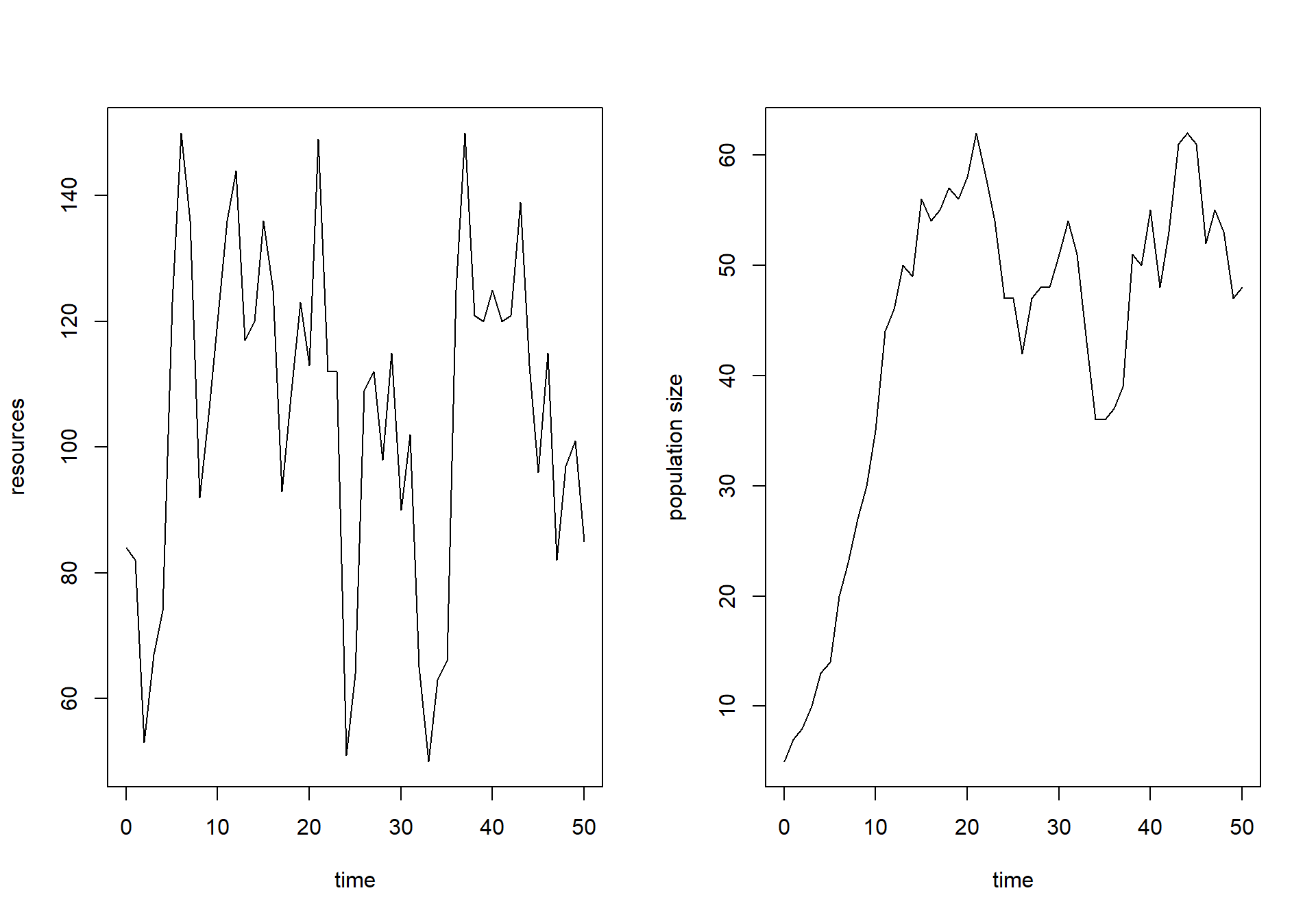
par(mfrow = c(1,1))InitLogistic that returns a named
vector with the initial value for state . Use the reserve’s ecologist’s estimate of
the initial state as the default value. Also define a function called
ParmsLogistic that returns a named vector with the
parameter values. Use the values measured above as default values.
# Function for the initial state values
InitLogistic <- function(N = 5) {
  # Gather function arguments in a named vector
  y <- c(N = N)

  # Return the named vector
  return(y)
}

# Function for the parameter values
ParmsLogistic <- function(r  = 0.25, # intrinsic population growth rate
                          k0 = 20,   # intercept of the carrying capacity
                          k1 = 0.2   # slope of the carrying capacity with R
                          ) {
  # Gather function arguments in a named vector
  y <- c(r = r,
         k0 = k0,
         k1 = k1)

  # Return the named vector
  return(y)
}R_linear, that
computes the value of resource as
function of time only. Use the approxfun function for this,
and the data loaded in surveyData. Use linear
interpolation. Use the forcing function to compute the linearly
interpolated value of resource at
time 13.4. # Create forcing function
R_linear <- approxfun(x = surveyData$t, y = surveyData$R, method = "linear", rule = 2)
# Apply forcing function to interpolate the value of R at time 13.4
R_linear(13.4)## [1] 118.2RatesLogistic that implements the
model and computes the rates of change of the state variable . Make sure to first interpolate the value
or as function of time by calling the
forcing function created above, then to compute , and then to compute the rate of change of
. Have the function return the values
of and as additional (or
auxiliary) information. # Function that returns the rate of change (and other information)
RatesLogistic <- function(t, y, parms) {
with(
as.list(c(y, parms)),{
# Optional: forcing functions: get value of the driving variables at time t (if any)
R <- R_linear(t)
# Optional: auxiliary equations
K <- k0 + k1 * R
# Rate equations
dNdt <- r * N * (1 - N/K)
# Gather all rates of change in a vector
# - the rates should be in the same order as the states (as specified in 'y')
RATES <- c(dNdt = dNdt)
# Optional: get in/out flow used to compute mass balances (or set MB <- NULL)
MB <- NULL
# Optional: gather auxiliary variables that should be returned (or set AUX <- NULL)
AUX <- c(R = R,
K = K)
# Return result as a list
outList <- list(c(RATES, # the rates of change of the state variables
MB), # the rates of change of the mass balance terms if MB is not NULL
AUX) # optional additional output per time step
return(outList)
}
)
}ode function, requesting output
at the times as specified in surveyData, and using the
“ode45” integration method. Save the output to an object called
states and plot the results (using the default plotting
method that produced line plots how the different variables change over
time). Also plot the simulated value of as function of time in a line plot, use
“time” as x-axis label and “population size” as y-axis label. Add the
measured values of the population’s measured size (column “N” in
surveyData) as points to the plot. # Numerically solve the model using the ode() function
states <- ode(y = InitLogistic(),
times = surveyData$t,
func = RatesLogistic,
parms = ParmsLogistic(),
method = "ode45")
plot(states)
# reset plotting window to 1 plot only
par(mfrow = c(1,1))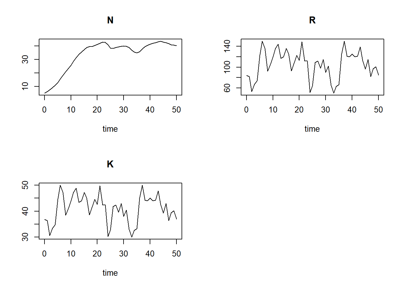
plot(states[,"time"], states[,"N"], type="l", xlab="time", ylab="N", ylim=c(0, 75))
points(surveyData$t, surveyData$N)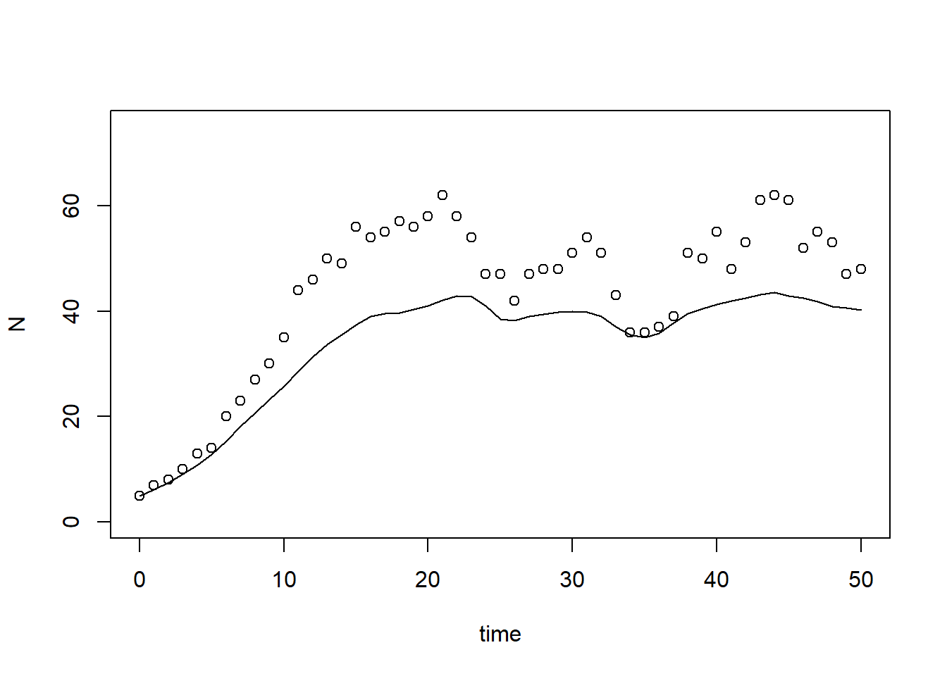
subset function to retrieve the output of the
simulation for time 50. states50 <- subset(states, time == 50)
states50## N R K
## 40.15437 85.00000 37.00000# also works:
# states[51,"N"]
# states[nrow(states),"N"]Exercise 7.2
Here, we use template 5 to compute the sensitivity index for state at times 5 and 50 while varying the parameters , and by 0.1%:
### Settings for sensitivity analysis

inits  <- InitLogistic()  # initial states
params <- ParmsLogistic() # parameters
times  <- surveyData$t    # times at which we request output
method <- "ode45"         # integration method

sensiParms <- c("r",      # the parameters to compute sensitivity indices for
                "k0",
                "k1")
                          # this can be a subset of all parameters

stateName <- "N"          # the state for which we want the sensitivity index

changeFraction <- 0.001   # the fraction by which each parameter is changed (here thus: 0.1%)
                          # (thus increased / decreased)

evalTime <- c(5, 50)      # time(s) for which we want to compute the sensitivity/elasticity indices


### Perform sensitivity analysis

# Create a data.frame to hold the output for each state in "sensiParms" and time in "evalTime" (stateDiff)
stateDiff <- data.frame(time = evalTime)
stateDiff[,stateName] <- NA
stateDiff[,sensiParms] <- NA

# Create empty vectors to hold the parameter differences (parmDiff)
parmDiff <- params[sensiParms] # this makes of copy of the named parameter vector
parmDiff[]  <- NA # This sets all elements within the vector to value NA

# Update the times vector with the value of evalTime (so that any evalTime is possible)
times <- sort(unique(c(times, evalTime)))

# In a 'for'-loop with iterator "i" (which values specfied by 'sensiParms'):
# - create 2 copies of 'params': called 'paramsLo' and 'paramsHi'
# - reduce the value of the i-th parameter in paramsLo with 'changeFraction'
# - increase the value of the i-th parameter in paramsHi with 'changeFraction'
# - solve the ODE model for both parameter sets (they are identical except for the i-th parameter)
# - get the values of the state after 'evalTime' time units and store the difference in 'stateDiff'
# - store the difference between the elevated and reduced parameter value in 'parmDiff'
for(i in sensiParms) {
  # Create copies of params
  paramsLo <- params
  paramsHi <- params

  # Reduce/increase the value of the i-th parameter
  paramsLo[i] <- (1 - changeFraction) * params[i]
  paramsHi[i] <- (1 + changeFraction) * params[i]

  # Solve the ODE model for both sets of parameters
  states_lo <- ode(y = inits,
                   times = times,
                   parms = paramsLo,
                   func = RatesLogistic,
                   method = method)
  states_hi <- ode(y = inits,
                   times = times,
                   parms = paramsHi,
                   func = RatesLogistic,
                   method = method)

  # Retrieve the values of the state variable at evalTime time units
  subsetLo <- subset(as.data.frame(states_lo), time %in% evalTime)[[stateName]]
  subsetHi <- subset(as.data.frame(states_hi), time %in% evalTime)[[stateName]]

  # Compute the differences and store in stateDiff
  stateDiff[,i] <- subsetHi - subsetLo

  # Store the difference between the elevated and reduced parameter value in the i-th element of parmDiff
  parmDiff[i] <- paramsHi[i] - paramsLo[i]
}

# the value of the state variable given the (unchanged!) parameter values
states <- ode(y = inits,
              times = times,
              parms = params,
              func = RatesLogistic,
              method = method)
stateDiff[,stateName] <- subset(as.data.frame(states), time %in% evalTime)[[stateName]]

### Compute sensitivity indices
SI <- stateDiff  # make copy of data.frame stateDiff
for(i in sensiParms) {
  SI[,paste("SI_d",i,sep="_")] <- stateDiff[,i] / parmDiff[i] # add index as new column
}

# inspect
SI
## time N r k0 k1 SI_d_r SI_d_k0 SI_d_k1
## 1 5 12.90815 0.020605991 0.00383273 0.002888567 41.21198 0.09581825 7.221417
## 2 50 40.15437 -0.005100951 0.04364429 0.037272083 -10.20190 1.09110719 93.180208Note here that the data.frame SI has columns:
- time (as specified in
evalTime, here 5 and 50); - state (name as specified in
stateName): value of the state with parameters at defaults (here N); - parameters listed in
sensiParms: the difference in the state when changing parameters one at a time (here: , , and ); - parameters listed in
sensiParmswith prefix “SI_d_”: the sensitivity index for each of the parameters (relative to the chosen state, here , at the chosen value for time t, here 5 or 50).
surveyData? See the computed sensitivity indices above in data.frame
SI, columns “SI_d_r”, “SI_d_k0”, “SI_d_k1” (At time 50,
state is most sensitive to changes in
parameter : if increases by 1 unit, then increases by ca. 93 units. This comes close
to the average value of resource :
mean(surveyData$R)## [1] 105.2745Realise that parameter is the slope of the relationship between and : thus if increases by 1 unit, then (on average!) increases by the average value of . As is the carrying capacity (although varying over time here), it is the value towards which the population size moves.
Initially, at short time scales (here time 5), the dynamical system is most sensitive to changes in the intrinsic growth rate (value of the index is ca. 41). This makes sense, as does not determine the (long term) carrying capacity, but rather the speed with which the population approaches .
With the information in SI, we can now compute the
elasticity of state N with respect to a change of parameter :
params["k1"] / SI$N * SI$SI_d_k1## [1] 0.1118893 0.4641100Per % of parameter , increases by about 0.11% at time 5 yet circa 0.46% at time 50.
We can compute the elasticity indices for the other parameters as well:
# Elasticity for r
params["r"] / SI$N * SI$SI_d_r
## [1] 0.79817773 -0.06351676# Elasticity for k0
params["k0"] / SI$N * SI$SI_d_k0## [1] 0.1484617 0.5434563# Elasticity for k1
params["k1"] / SI$N * SI$SI_d_k1## [1] 0.1118893 0.4641100The elasticity index is the highest for at time 5: per % change in , changes by almost 0.8%.
Solutions as R script
Download here the code as shown on this page in a separate .r file.