Wageningen University & Research | FEM-31806 | Models for Ecological Systems | FEM | PPS | WEC
GPLakeR - Day 4
First make a copy of the script you created on Day 2 to implemented the model (or, copy the solution of the implementation of the model from the solution to day 2, and then continue with the exercises below.
Aims
Aim 1: Sensitivity
Probably you have already separated parameters between those that are true constants (e.g. molar weights, physical properties etc.), those that are more or less invariable or are measured with great precision and therefore hard coded in the parameter list, and those that are highly uncertain and/or can vary a lot in different scenarios. The latter are in this course typically defined per scenario and given as input arguments to the function creating a named vector with parameter values, or as a defined list in input scenario-specific input files for other models.
Select three parameters for sensitivity analysis. Run both a sensitivity analysis (sensu stricto), and also an elasticity analysis, which is a normalized version of sensitivity (see textbook and lectures for differences). Run the model three times (2000 days) but with different parameter values: at the default parameter value, at the default parameter value -10%, and at the default parameter value +10%. Study the effects of these parameter values for the state variables: sPmacr. Visualize by plotting the results. For visualization you can first best plot the state variable(s) of interest against time (possibly with multiple scenarios in a single plot; a separate line for each scenario). Moreover, you can opt for a barplot showing the sensitivity and elasticity index values for the parameters.
In the GPLakeR model, the state variables can possibly end up in alternative stable states, dependent on an increase or decrease in nutrient values (parameter
Pload). For running the analysis, we advise running the model for 25000 days, starting with aPloadof 0.05, and increasingPloadlinearly from 0.05 (gPm-3) to 5 from day 5000 to day 15000, and from 5 to 0.05 from day 15000 to day 25000. Define for this dynamics inPloada simple data.frame with 2 columns (timeandPload) and 4 rows with their values, then use theapproxfunfunction to create a forcing function so that you can interpolate the value ofPloadat the current timetin the integration in theRatesGPLakeRfunction (work in a copy of theRatesGPLakeRfunction and call itRatesGPLakeRforcing- see template 2). Initialize with values valuessPmacr = 250,sPphyt = 0,sPwater = 0, and set parameterDto value 0.01 (all others at their default values). At whatPloaddoes the system switch? What are the critical P loadings?
Aim 2: Calibration
- Calibrate the model for three critical and uncertain parameters: Pload. Use the data sets provided on Brightspace (GPLakeR.csv). Calibrate the model for state variable sPmacr, using the numerical optimization method as developed in Template 6. Visualize the implications for the model: plot the state variables against time.
Aim 3: Validation
Give the options to validate your model.
What data would you need?
Answers
Download here the code as shown on this page in a separate .r file.
Sensitivity
Parameters
The function returning a named vector with parameter values:
ParmsGPLakeR <- function(
    Pload = 2, # Areal P loading (mg P.m-2.d-1)
    z = 2, # Depth (m)
    D = 0.01, # Dilution rate (d-1)
    Rmacr = 0.004, # Macrophyte nutrient retention rate (d-1)
    Rphyt = 0.01, # Phytoplankton nutrient retention rate (d-1)
    Mmacr = 250, # Areal P content of macrophytes at equilibrium during light-limitation (mg P.m-2)
    Mphyt = 250, # Areal P content of phytoplankton at equilibrium during light-limitation (mg P.m-2)
    Gmacr = 0.1, # Maximum per capita growth rate of macrophytes (d-1)
    Gphyt = 0.1, # Maximum per capita growth rate of phytoplankton (d-1)
    Hmacrnutr = 0.01, # Half-saturation constant of nutrient limitation of macrophytes (mg P.m-3)
    Hphytnutr = 0.1, # Half-saturation constant of nutrient limitation of phytoplankton (mg P.m-3)
    Pcrit = 70, # Critical turbidity (mg P.m-2)
    nIntlog = 3, # Parameter in intlog function (-)
    nHill = 30, # Parameter in Hill function (-)
    inocmacr = 0.000001, # Inoculum of macrophytes (mg P.m-2)
    inocphyt = 0.000001, # Inoculum of phytoplankton (mg P.m-2)
    inocratemacr = 0.000001, # Inoculum rate of macrophytes (mg P.m-2.d-1)
    inocratephyt = 0.000001 # Inoculum rate of phytoplankton (mg P.m-2.d-1)
    ) {

  # Gather function arguments in a named vector
  y <- c(Pload = Pload,
         z = z,
         D = D,
         Rmacr = Rmacr,
         Rphyt = Rphyt,
         Mmacr = Mmacr,
         Mphyt = Mphyt,
         Gmacr = Gmacr,
         Gphyt = Gphyt,
         Hmacrnutr = Hmacrnutr,
         Hphytnutr = Hphytnutr,
         Pcrit = Pcrit,
         nIntlog = nIntlog,
         nHill = nHill,
         inocmacr = inocmacr,
         inocphyt = inocphyt,
         inocratemacr = inocratemacr,
         inocratephyt = inocratephyt)

  # Return
  return(y)
}
Initial conditions
The function returning a named vector with initial values for the 3 state variables:
- sPmacr: Areal P content of macrophytes (mg P.m-2);
- sPphyt: Areal P content of phytoplankton (mg P.m-2);
- sPwater: (Free) P concentration in the water (mg P.m-3):
InitGPLakeR <- function(
    sPmacr = 250, # Areal P content of macrophytes (mg P.m-2)
    sPphyt = 0, # Areal P content of phytoplankton (mg P.m-2)
    sPwater = 0 # (Free) P concentration in the water (mg P.m-3)
    ) {

  # Gather initial conditions in a named vector; given names are names for the state variables in the model
  y <- c(sPmacr = sPmacr,
         sPphyt = sPphyt,
         sPwater = sPwater)

  # Return
  return(y)
}
Differential equations
The function computing the rates of change of the state variables with respect to time:
RatesGPLakeR <- function(t, y, parms) {
  # use the with() function to be able to access the parameters and states easily
  # remember that the with() function is with(data, expr), where
  # - 'data' is ideally a list with named elements
  #   thus: 'y' and 'parms' are combined using function c and converted using function as.list
  # - 'expr' is an expression (i.e. code) that is evaluated
  #   this can span multiple lines of code when embraced with curly brackets {}
  with(
    as.list(c(y, parms)),{

      ### Optional: forcing functions: get value of the driving variables at time t (if any)

      ### Optional: auxiliary equations
      Pwater <- max(sPwater, 0)
      LRmacr <- Mmacr * ( 1 - log(exp(nIntlog * (1 - Pload / (Rmacr * Mmacr))) + 1) / log(exp(nIntlog) + 1))
      LRphyt <- Mphyt * (1 - log(exp(nIntlog * (1 - Pload / ((Rphyt + D) * Mphyt))) + 1) / log(exp(nIntlog) + 1))
      State <- Pcrit ^ nHill / (Pcrit ^ nHill + sPphyt ^ nHill)
      Pmacreq <- LRmacr * State
      Pphyteq <- min(max(((Pload - Rmacr * sPmacr) / (Rphyt + D)),0),LRphyt) * State + LRphyt * (1 - State)
      Pwatereq <- ((Pload - (Rphyt + D) * LRphyt) / (z * D)) * (1 - State)
      Macrnutrlim <- Pwater / (Hmacrnutr + Pwater)
      Phytnutrlim <- Pwater / (Hphytnutr + Pwater)
      Hmacrdens <- Rmacr / (Gmacr - Rmacr) # H for density dependence of macrophytes
      Hphytdens <- (Rphyt + D) / (Gphyt - (Rphyt + D)) # H for density dependence of phytoplankton
      Macrdenslim <- Hmacrdens / (Hmacrdens + sPmacr / (Pmacreq + inocmacr))
      Phytdenslim <- Hphytdens / (Hphytdens + sPphyt / (Pphyteq + inocphyt))
      GRmacr <- Gmacr * Macrnutrlim * Macrdenslim
      GRphyt <- Gphyt * Phytnutrlim * Phytdenslim

      # Rate equations
      dPmacr <- inocratemacr + GRmacr * sPmacr - Rmacr * sPmacr
      dPphyt <- inocratephyt + GRphyt * sPphyt - (Rphyt + D) * sPphyt
      dPwater <- (Pload - GRmacr * sPmacr - GRphyt * sPphyt) / z - D * Pwater

      ### Gather all rates of change in a vector
      # - the rates should be in the same order as the states (as specified in 'y')
      # - it can be a named vector, but does not need to be
      RATES <- c(dPmacr = dPmacr,
                 dPphyt = dPphyt,
                 dPwater = dPwater)

      ### Optional: get in/out flow used to compute mass balances (or set MB <- NULL)
      # not included here (thus here use MB <- NULL), see template 3
      MB <- NULL

      ### Optional: gather auxiliary variables that should be returned (or set AUX <- NULL)
      # - this should be a named vector or list!
      AUX <- NULL

      # Return result as a list
      # - the first element is a vector with the rates of change (in the same order as 'y')
      # - all other elements are (optional) extra output, which should be named
      outList <- list(c(RATES, # the rates of change of the state variables (same order as 'y'!)
                        MB),   # the rates of change of the mass balance terms (or NULL)
                      AUX) # optional additional output per time step
      return(outList)
    })
}
With these 3 functions now defined, the GPLakeR mini-model has been
implemented in R code, and the model can now numerically be solved using
the ode function from the deSolve package.
Here, let’s solve the model for 3 different values of parameter
Pload: first for its default value (2; solved model stored
in states), then when increasing it by 10% (solved model
stored in statesHI), and then when decreasing it with 10%
(solved model stored in statesLO).
states <- ode(y = InitGPLakeR(),
              times = seq(from = 0, to = 2000, by = 20),
              func = RatesGPLakeR,
              parms = ParmsGPLakeR(Pload = 2),
              method = "ode45")
statesHI <- ode(y = InitGPLakeR(),
                times = seq(from = 0, to = 2000, by = 20),
                func = RatesGPLakeR,
                parms = ParmsGPLakeR(Pload = 1.1*2),
                method = "ode45")
statesLO <- ode(y = InitGPLakeR(),
                times = seq(from = 0, to = 2000, by = 20),
                func = RatesGPLakeR,
                parms = ParmsGPLakeR(Pload = 0.9*2),
                method = "ode45")
We can show these different scenarios:
plot(states, statesHI, statesLO)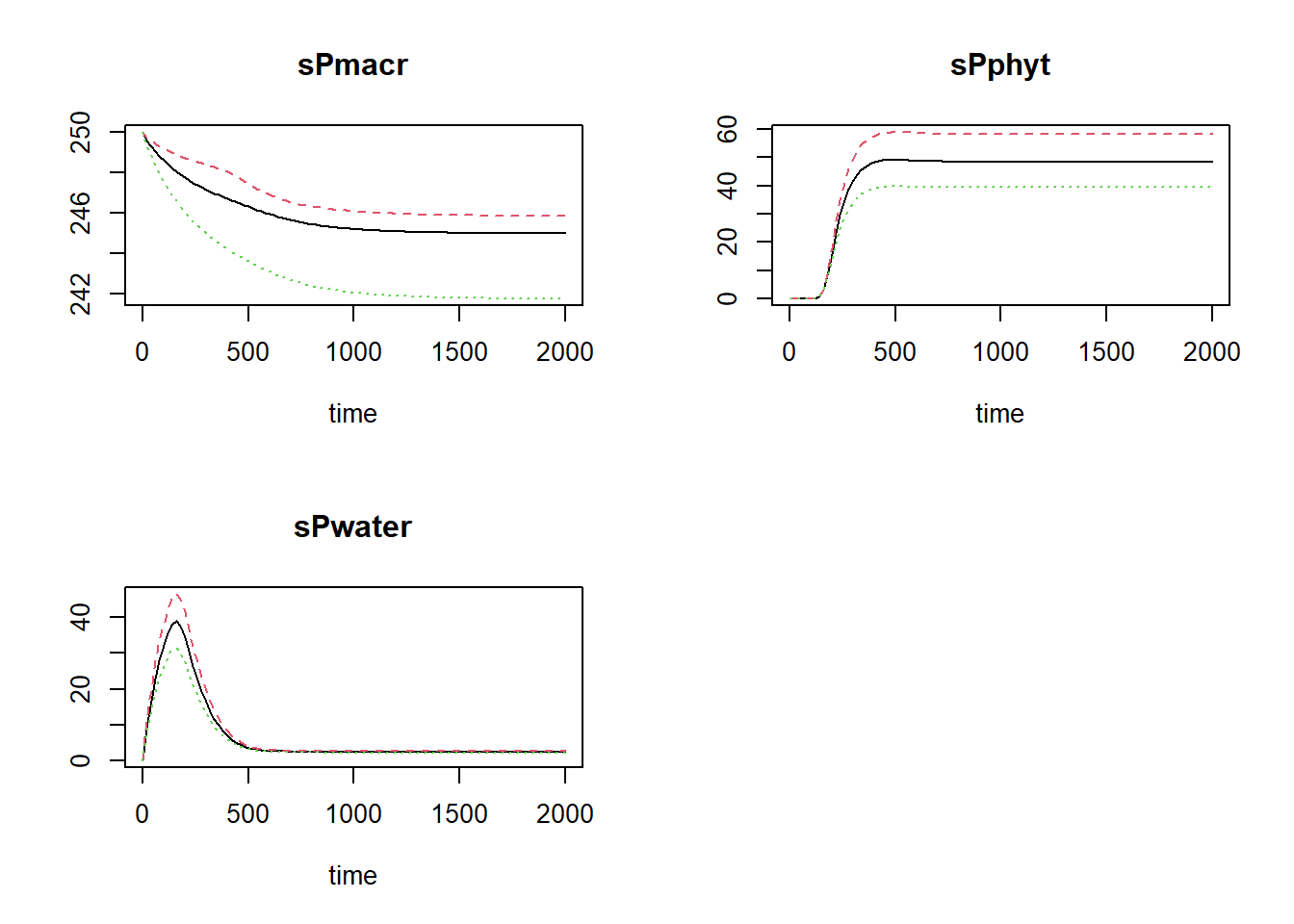
where the black line is the default value for Pload, the
red line is the high value (10% increase), and the green line shows the
simulation for the value reduced by 10%.
We can now calculate the sensitivity index (SI) and elasticity index
(EI) of the parameter Pload on state sPmacr at
the end of the simulation:
deltaState = statesHI[nrow(statesHI),"sPmacr"] - statesLO[nrow(statesHI),"sPmacr"]
deltaParm = 0.1*2
SI <- deltaState / (2*deltaParm)
SI
## sPmacr
## 10.25035EI <- (deltaState/states[nrow(states),"sPmacr"]) / ((2*deltaParm) / 2)
EI## sPmacr
## 0.08368095This approach can be repeated for the other parameters and both state variables. Repeating the same procedure for all parameters and all state variables yields the following elasticity indices:
### Settings for sensitivity analysis

# integration settings
inits <- InitGPLakeR()
parms <- ParmsGPLakeR()
times <- seq(from = 0, to = 2000, by = 20)
method <- "ode45"

# Specify the parameters to compute sensitivity indices for
sensiParms <- names(parms) # this can be a subset of all parameters

# Set the fraction by which each parameter is decreased/increased during sensitivity analysis
changeFraction <- 0.1 # 10%

# Set the time at which we want to evaluate the values of the state variables
evalTime <- max(times) # this can be e.g. max(times): it can also be other times, but MUST occur in 'times'!

# Set the name of the state variable for which we want to compute the sentitivity index
stateName <- "sPmacr"


### Perform sensitivity analysis

# Create data.frame to hold the output for each state in "sensiParms" and time in "evalTime" (stateDiff)
stateDiff <- data.frame(time = evalTime)
stateDiff[,stateName]  <- NA # Column for the value of the state given the unchanged parameters
stateDiff[,sensiParms] <- NA # Column(s) for the difference in state values given changes in parameters

# Create empty vectors to hold the parameter differences (parmDiff)
parmDiff <- parms[sensiParms] # this makes of copy of the named parameter vector
parmDiff[]  <- NA # This sets all elements within the vector to value NA

# Update the times vector with the value of evalTime (so that any evalTime is possible)
times <- sort(unique(c(times, evalTime)))

# In a 'for'-loop with iterator "i" (which values specfied by 'sensiParms'):
# - create 2 copies of 'parms': called 'paramsLo' and 'paramsHi'
# - reduce the value of the i-th parameter in paramsLo with 'changeFraction'
# - increase the value of the i-th parameter in paramsHi with 'changeFraction'
# - solve the ODE model for both parameter sets (they are identical except for the i-th parameter)
# - get the values of the state after 'evalTime' time units and store the difference in 'stateDiff'
# - store the difference between the elevated and reduced parameter value in 'parmDiff'
for(i in sensiParms) {
  # Create copies of parms
  paramsLo <- parms
  paramsHi <- parms

  # Reduce/increase the value of the i-th parameter
  paramsLo[i] <- (1 - changeFraction) * parms[i]
  paramsHi[i] <- (1 + changeFraction) * parms[i]

  # Solve the ODE model for both sets of parameters
  states_lo <- ode(y = inits,
                   times = times,
                   parms = paramsLo,
                   func = RatesGPLakeR,
                   method = method)
  states_hi <- ode(y = inits,
                   times = times,
                   parms = paramsHi,
                   func = RatesGPLakeR,
                   method = method)

  # Retrieve the values of the state variable at evalTime time units
  subsetLo <- subset(as.data.frame(states_lo), time %in% evalTime)[[stateName]]
  subsetHi <- subset(as.data.frame(states_hi), time %in% evalTime)[[stateName]]

  # Compute the differences and store in stateDiff
  stateDiff[,i] <- subsetHi - subsetLo

  # Store the difference between the elevated and reduced parameter value in the i-th element of parmDiff
  parmDiff[i] <- paramsHi[i] - paramsLo[i]
}

# Add the value of the state variable given the (unchanged!) parameter values
states <- ode(y = inits,
              times = times,
              parms = parms,
              func = RatesGPLakeR,
              method = method)
stateDiff[,stateName] <- subset(as.data.frame(states), time %in% evalTime)[[stateName]]

### Compute sensitivity indices
SI <- stateDiff  # make copy of data.frame stateDiff
for(i in sensiParms) {
  SI[,paste("SI_d",i,sep="_")] <- stateDiff[,i] / parmDiff[i] # add index as new column
}
We can now inspect the sensitivity index:
SI## time sPmacr Pload z D Rmacr Rphyt Mmacr Mphyt Gmacr Gphyt Hmacrnutr Hphytnutr Pcrit nIntlog
## 1 2000 244.9864 4.100138 -0.1038395 -0.07146018 -4.712618 0.03203514 44.17854 -3.726386e-06 0.00833426 -0.02710324 -0.2041238 0.1010331 0.1014127 3.146827
## nHill inocmacr inocphyt inocratemacr inocratephyt SI_d_Pload SI_d_z SI_d_D SI_d_Rmacr SI_d_Rphyt SI_d_Mmacr SI_d_Mphyt SI_d_Gmacr
## 1 0.01133451 1.98738e-07 -4.028252e-08 5.407035e-05 -3.547486e-05 10.25035 -0.2595987 -35.73009 -5890.772 16.01757 0.8835708 -7.452772e-08 0.416713
## SI_d_Gphyt SI_d_Hmacrnutr SI_d_Hphytnutr SI_d_Pcrit SI_d_nIntlog SI_d_nHill SI_d_inocmacr SI_d_inocphyt SI_d_inocratemacr SI_d_inocratephyt
## 1 -1.355162 -102.0619 5.051653 0.007243765 5.244711 0.001889084 0.9936899 -0.2014126 270.3518 -177.3743We can also calculate the elasticity indices, rounded to 5 digits and sorted on decreasing absolute value:
Es <- parms[sensiParms] / SI$sPmacr * SI[,paste("SI_d",sensiParms,sep="_")]
Es <- as.numeric(Es)
names(Es) <- sensiParms
round(Es[order(abs(Es),decreasing=TRUE)],5)
## Mmacr Rmacr Pload nIntlog Hmacrnutr z Pcrit Hphytnutr D Rphyt Gphyt nHill
## 0.90165 -0.09618 0.08368 0.06422 -0.00417 -0.00212 0.00207 0.00206 -0.00146 0.00065 -0.00055 0.00023
## Gmacr inocratemacr inocratephyt Mphyt inocmacr inocphyt
## 0.00017 0.00000 0.00000 0.00000 0.00000 0.00000We could use a barplot to show the elasticities:
barplot(Es, col = 1:8, beside = TRUE)
legend(x="topright", horiz=FALSE, bty="n", legend=names(Es), pch=22, cex=0.7, col=1:8)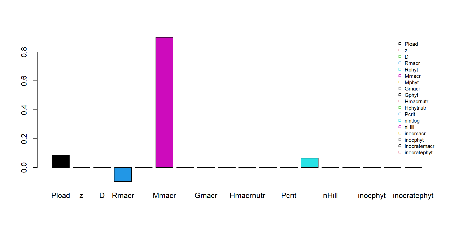
To include a time-varying parameter Pload, we can use
the approxfun function to create a forcing function that
can be used within the RatesGPLakeR function to interpolate
the value of Pload. First create a data.frame with the
columns time (values 0, 5000, 15000 and 25000) and
Pload (values 0.05, 0.05, 5 and 0.05):
Ploaddf <- data.frame(time = c(0, 5000, 15000, 25000),
                      Pload = c(0.05, 0.05, 5, 0.05))
Ploaddf
## time Pload
## 1 0 0.05
## 2 5000 0.05
## 3 15000 5.00
## 4 25000 0.05Using the data.frame Ploadf we can now create the
forcing function, and test it by plotting:
Pload_forcingfunction <- approxfun(x = Ploaddf$time, y = Ploaddf$Pload, method = "linear", rule = 2)
plot(0:25000, Pload_forcingfunction(0:25000), type = "l", xlab = "time", ylab = "Pload")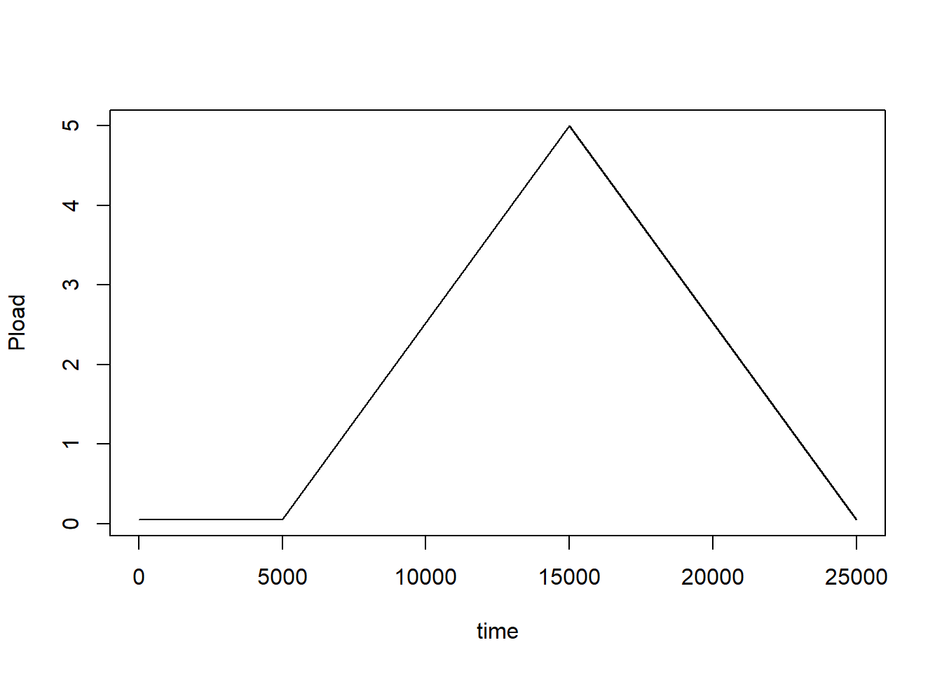
Now, we can update the RatesGPLakeR function (let’s
create a copy to call it RatesGPLakeRforcing), to include
the forcing function Pload_forcingfunction that will be
evaluated at time t to compute parameter
Pload. The computed value for Pload is also
returned as an auxiliary variable:
RatesGPLakeRforcing <- function(t, y, parms) {
  # use the with() function to be able to access the parameters and states easily
  # remember that the with() function is with(data, expr), where
  # - 'data' is ideally a list with named elements
  #   thus: 'y' and 'parms' are combined using function c and converted using function as.list
  # - 'expr' is an expression (i.e. code) that is evaluated
  #   this can span multiple lines of code when embraced with curly brackets {}
  with(
    as.list(c(y, parms)),{

      ### Optional: forcing functions: get value of the driving variables at time t (if any)
      Pload <- Pload_forcingfunction(t)

      ### Optional: auxiliary equations
      Pwater <- max(sPwater, 0)
      LRmacr <- Mmacr * ( 1 - log(exp(nIntlog * (1 - Pload / (Rmacr * Mmacr))) + 1) / log(exp(nIntlog) + 1))
      LRphyt <- Mphyt * (1 - log(exp(nIntlog * (1 - Pload / ((Rphyt + D) * Mphyt))) + 1) / log(exp(nIntlog) + 1))
      State <- Pcrit ^ nHill / (Pcrit ^ nHill + sPphyt ^ nHill)
      Pmacreq <- LRmacr * State
      Pphyteq <- min(max(((Pload - Rmacr * sPmacr) / (Rphyt + D)),0),LRphyt) * State + LRphyt * (1 - State)
      Pwatereq <- ((Pload - (Rphyt + D) * LRphyt) / (z * D)) * (1 - State)
      Macrnutrlim <- Pwater / (Hmacrnutr + Pwater)
      Phytnutrlim <- Pwater / (Hphytnutr + Pwater)
      Hmacrdens <- Rmacr / (Gmacr - Rmacr) # H for density dependence of macrophytes
      Hphytdens <- (Rphyt + D) / (Gphyt - (Rphyt + D)) # H for density dependence of phytoplankton
      Macrdenslim <- Hmacrdens / (Hmacrdens + sPmacr / (Pmacreq + inocmacr))
      Phytdenslim <- Hphytdens / (Hphytdens + sPphyt / (Pphyteq + inocphyt))
      GRmacr <- Gmacr * Macrnutrlim * Macrdenslim
      GRphyt <- Gphyt * Phytnutrlim * Phytdenslim

      # Rate equations
      dPmacr <- inocratemacr + GRmacr * sPmacr - Rmacr * sPmacr
      dPphyt <- inocratephyt + GRphyt * sPphyt - (Rphyt + D) * sPphyt
      dPwater <- (Pload - GRmacr * sPmacr - GRphyt * sPphyt) / z - D * Pwater

      ### Gather all rates of change in a vector
      # - the rates should be in the same order as the states (as specified in 'y')
      # - it can be a named vector, but does not need to be
      RATES <- c(dPmacr = dPmacr,
                 dPphyt = dPphyt,
                 dPwater = dPwater)

      ### Optional: get in/out flow used to compute mass balances (or set MB <- NULL)
      # not included here (thus here use MB <- NULL), see template 3
      MB <- NULL

      ### Optional: gather auxiliary variables that should be returned (or set AUX <- NULL)
      # - this should be a named vector or list!
      AUX <- c(Pload = Pload)

      # Return result as a list
      # - the first element is a vector with the rates of change (in the same order as 'y')
      # - all other elements are (optional) extra output, which should be named
      outList <- list(c(RATES, # the rates of change of the state variables (same order as 'y'!)
                        MB),   # the rates of change of the mass balance terms (or NULL)
                      AUX) # optional additional output per time step
      return(outList)
    })
}
Now, we can solve this model with the initial values sPmacr = 250, sPphyt = 0, sPwater = 0, and the parameter D = 0.01 (all others at their default values) for 25000 time-steps (note that this may take a little while):
statesPload1 <- ode(y = InitGPLakeR(sPmacr = 5, sPphyt = 0, sPwater = 0),
                  times = seq(from = 0, to = 25000, by = 1),
                  parms = ParmsGPLakeR(D = 0.01),
                  func = RatesGPLakeRforcing,
                  method = "ode45")
plot(statesPload1)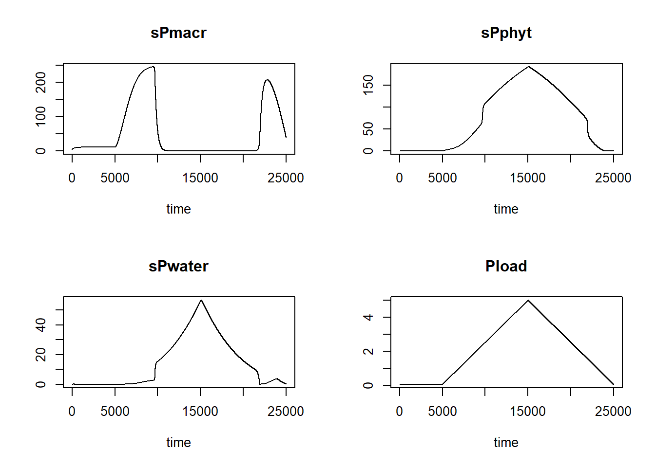
We can now also plot Pload against sPmacr:
plot(statesPload1[,"Pload"], statesPload1[,"sPmacr"], xlab = "Pload", ylab = "sPmacr", type = "l")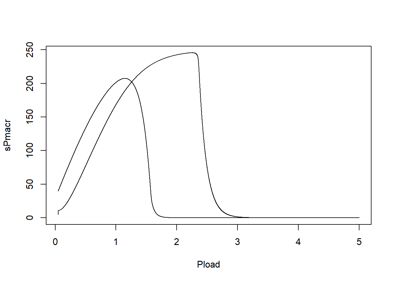
In such a plot, we can see that the system has alternative stable states: with increasing P loading, the lake can stay in a clear and vegetated state for quite long, up to a point where P loading becomes too high (ca. 2.3) so that the lake suddenly switches to a turbid state without vegetation (the state sPmacr does not become mathematically 0, but it will become very low). After this switching point, when we reduce P loading, the system does not suddenly switch back at the same level of P loading: it has to drop to a lower value (ca. 1.8) before the system switches back to a clear and vegetation state.
Calibration
First, load the data from the file GPLakeR.csv (e.g. stored in the data folder):
dat <- read.csv("data/GPLakeR.csv")Explore the data by showing the header of the file:
head(dat)## time sPmacr sPphyt sPwater
## 1 0 48.31 37.80 138.36
## 2 100 92.73 70.69 17.10
## 3 200 105.73 69.88 2.30
## 4 300 119.77 59.39 0.59
## 5 400 151.83 57.56 0.74
## 6 500 179.76 55.04 0.97We see the values of the state variables at time 0, so assume that these are the initial values of the states, to be used below in the simulation of the models:
inits = c(sPmacr = 48.31, sPphyt = 37.80, sPwater = 138.36)Let’s first simulate the model with default parameter values and these initial state value, and check how well the modelled predictions for “sPmacr” agree with the measured values for state “sPmacr”:
# Simulate with default parameter values
states <- ode(y = inits,
              times = seq(from = 0, to = max(dat$time), by = 1),
              parms = ParmsGPLakeR(),
              func = RatesGPLakeR,
              method = "ode45")
# Plot
plot(states[,"time"], states[,"sPmacr"], type="l", xlab="Time", ylab="State sPmacr", ylim=c(0,250))
points(dat$time, dat$sPmacr, pch=16)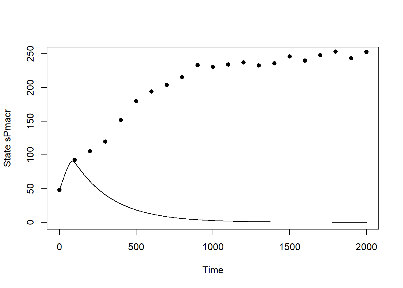
In order to calibrate the model, we first have to define a few
functions (predictionError, predRMSE,
transformParameters and calibrateParameters)
that allow us to do the calibration. These functions can be found in
template 6. Note that we do not have to fill something in here: we only
are defining these functions as is, and later when we
call (use) these functions we have to supply them with the
appropriate inputs.
First, function predictionError (copy from template
6):
# Define a function that computes prediction errors
# NOTE: nothing needs to be filled in here, so this function can be used as-is
# (unless there is a need to change it, e.g. change the solver method, or include events etc.)
predictionError <- function(p,          # the parameters
                            y0,         # the initial conditions
                            fn,         # the function with rate equation(s)
                            name,       # the name of the state parameter
                            obs_values, # the measured state values
                            obs_times,  # the time-points of the measured state values
                            out_time = seq(from = 0, # times for the numerical integration
                                           to = max(obs_times), # default: 0 - max(obs_times)
                                           by = 1) # in steps of 1
                            ) {
  # Get out_time vector to retrieve predictions for (combining 'obs_times' and 'out_time')
  out_time <- unique(sort(c(obs_times, out_time)))

  # Solve the model to get the prediction
  pred <- ode(y = y0,
              times = out_time,
              func = fn,
              parms = p,
              method = "ode45")
  # NOTE: in case of a 'stiff' problem, method "ode45" might result in an error that the max nr of
  # iterations is reached. Using method "rk4" (fixed timestep 4th order Runge-Kutta) might solve this.

  # Get predictions for our specific state, at times t
  pred_t <- subset(pred, time %in% obs_times, select = name)

  # Compute errors, err: prediction - obs
  err <- pred_t - obs_values

  # Return
  return(err)
}
Second, function predRMSE (copy from template 6):
# Define a function that computes the Root Mean Squared Error, RMSE
# NOTE: nothing needs to be filled in here, so this function can be used as-is
predRMSE <- function(...) { # NOTE: these ... are ellipsis, so DO NOT fill in something here!
  # Get prediction errors
  err <- predictionError(...) # NOTE: these ... are ellipsis, so DO NOT fill in something here!

  # Compute the measure of model fit (here the Root Mean Squared Error)
  RMSE <- sqrt(mean(err^2))

  # Return the measure of model fit
  return(RMSE)
}
Third, function transformParameters (copy from template
6):
# Define a function that allows for transformation and back-transformation
# NOTE: nothing needs to be filled in here, so this function can be used as-is
transformParameters <- function(parm, trans, rev = FALSE) {
  # Check transformation vector
  trans <- match.arg(trans, choices = c("none","logit","log"), several.ok = TRUE)

  # Get transformation function per parameter
  if(rev == TRUE) {
    # Back-transform from real scope to parameter scope
    transfun <- sapply(trans, switch,
                       "none" = mean,
                       "logit" = plogis,
                       "log" = exp)
  }else {
    # Transform from parameter scope to real scope
    transfun <- sapply(trans, switch,
                       "none" = mean,
                       "logit" = qlogis,
                       "log" = log)
  }

  # Apply transformation function
  y <- mapply(function(x, f){f(x)}, parm, transfun)

  # Return
  return(y)
}
And fourth, function calibrateParameters (copy from
template 6):
# Define a function that performs the calibration of specified parameters
# NOTE: nothing needs to be filled in here, so this function can be used as-is
calibrateParameters <- function(par,  # parameters
                                init, # initial state values
                                fun,  # function that returns the rates of change
                                stateCol, # name of the state variable
                                obs,  # observed values of the state variable
                                t,    # timepoints of the observed state values
                                calibrateWhich, # names of the parameters to calibrate
                                transformations, # transformation per calibration parameter
                                times = seq(from = 0, # times for the numerical integration
                                            to = max(t), # default: 0 - max(t)
                                            by = 1), # in steps of 1
                                ... # NOTE: these ... are ellipsis, so DO NOT fill in something here!
                                    # these are the optional extra arguments past on to optim()
                                ) {
  # check names of parameters that need calibration
  calibrateWhich <- match.arg(calibrateWhich, choices = names(par), several.ok = TRUE)

  # Create vector with transformations for all parameters (set to "none")
  tranforms <- rep("none", length(par))
  names(tranforms) <- names(par) # set the names of each transformation

  # Overwrite the elements for parameters that need calibration
  tranforms[calibrateWhich] <- transformations

  # Transform parameters
  par <- transformParameters(parm = par, trans = tranforms, rev = FALSE)

  # Get parameters to be estimated
  par_fit <- par[calibrateWhich]

  # Specify the cost function: the function that will be optimized for the parameters to be estimated
  costFunction <- function(parm_optim, parm_all,
                           init, fun, stateCol, obs, t,
                           times = t,
                           optimNames = calibrateWhich,
                           transf = tranforms,
                           ... # NOTE: these ... are ellipsis, so DO NOT fill in something here!
                           ) {
    # Gather parameters (those that are and are not to be estimated)
    par <- parm_all
    par[optimNames] <- parm_optim[optimNames]

    # Back-transform
    par <- transformParameters(parm = par, trans = transf, rev = TRUE)

    # Get RMSE
    y <- predRMSE(p = par, y0 = init, fn = fun,
                  name = stateCol, obs_values = obs, obs_times = t,
                  out_time = times)

    # Return
    return(y)
  }

  # Fit using optim
  fit <- optim(par = par_fit,
               fn =  costFunction,
               parm_all = par,
               init = init,
               fun = fun,
               stateCol = stateCol,
               obs = obs,
               t = t,
               times = times,
               ...) # NOTE: these ... are ellipsis, so DO NOT fill in something here!
                    # These are the optional additional arguments passed on to optim()

  # Gather parameters: all parameters updated with those that are estimated
  y <- par
  y[calibrateWhich] <- fit$par[calibrateWhich]

  # Back-transform
  y <- transformParameters(parm = y, trans = tranforms, rev = TRUE)

  # put all (constant and estimated) parameters back in $par
  fit$par <- y

  # Add the calibrateWhich information
  fit$calibrated <- calibrateWhich

  # return 'fit'object:
  return(fit)
}
After defining these 4 functions, we can get started with the actual calibration. For this we need to make some choices, e.g. which parameters to calibrate, and what are the transformations needed (no transformation, logarithmic transformation, or logit transformation, see explanation in template 6). Because all parameters in this model should be positive, let’s use a log-transform in the calibration routine.
Let’s calibrate only the parameters “Pload”,“Rmacr” and “D” of the
GPLakeR model, based on the dataset dat and the
measurements (and thus state) “sPmacr”. We only have to simulate to the
maximum time of our dataset dat (thus
max(dat$t)). As initial state values we use the
inits as defined above (the first row of dat).
Note that the calibration may take some time (several seconds/minutes)
to complete:
# Perform the calibration
fit <- calibrateParameters(par = ParmsGPLakeR(),
                           init = inits,
                           fun = RatesGPLakeR,
                           stateCol = "sPmacr",
                           obs = dat$sPmacr,
                           t = dat$time,
                           times = seq(from = 0, to = max(dat$time), by = 1),
                           calibrateWhich = c("Pload","Rmacr","D"),
                           transformations = c("log","log","log"))
We can retrieve information on the model fitting by looking at the
object fit:
fit## $par
## Pload z D Rmacr Rphyt Mmacr Mphyt Gmacr Gphyt Hmacrnutr Hphytnutr Pcrit
## 2.001280e+00 2.000000e+00 1.404934e-02 3.020011e-03 1.000000e-02 2.500000e+02 2.500000e+02 1.000000e-01 1.000000e-01 1.000000e-02 1.000000e-01 7.000000e+01
## nIntlog nHill inocmacr inocphyt inocratemacr inocratephyt
## 3.000000e+00 3.000000e+01 1.000000e-06 1.000000e-06 1.000000e-06 1.000000e-06
##
## $value
## [1] 4.047461
##
## $counts
## function gradient
## 412 NA
##
## $convergence
## [1] 0
##
## $message
## NULL
##
## $calibrated
## [1] "Pload" "Rmacr" "D"Explanation of these outputs are given in the optimization function explanation of Template 6:
- “par”: the calibrated parameter values. This includes all model parameters: those that are kept constant as well as those that have been calibrated;
- “value”: this is the value of the cost-function at the values as given in “par”. Here, this is thus the RMSE of the model predictions given the parameter values in “par”;
- “counts”: information about the number of iterations that the
optimfunction needed; - “convergence”: information about the convergence of the
optimfunction: a value of 0 means that the estimation successfully converged! For other values, see?optimfor the help-documentation of theoptimfunction; - “message”: a character string giving any additional information
returned by the optimizer, or
NULL; - “calibrated”: a character string with the model parameters that have
been calibrated (thus the vector passed as input to argument
calibrateWhich).
Then, we can use the fitted/calibrated model parameters (object
fit$par) to simulate the model, and plot the result:
# Fit the model using the calibrated values
statesFitted <- ode(y = inits,
                    times = seq(from=0, to = max(dat$time), by = 1),
                    parms = fit$par,
                    func = RatesGPLakeR,
                    method = "ode45")
plot(statesFitted)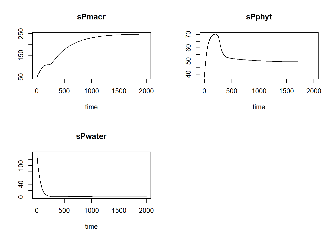
Also, we can plot the modelled pattern of state “sPmacr” as function of time, including the measured values of “sPmacr”:
plot(statesFitted[,"time"], statesFitted[,"sPmacr"], type = "l", xlab = "Time", ylab = "State sPmacr")
points(dat$time, dat$sPmacr, pch=16)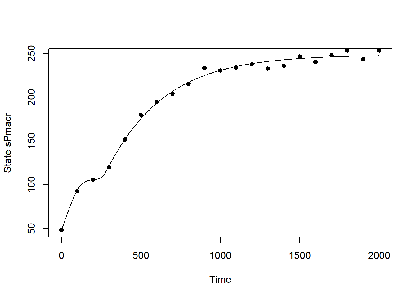
The calibrated model seems to capture the observed pattern quite well! In order to quantify the difference between the calibrated model and the model solved with default parameter values, let’s compute the RMSE for both models:
predRMSE(p = ParmsGPLakeR(),
         y0 = inits,
         fn = RatesGPLakeR,
         name = "sPmacr",
         obs_values = dat$sPmacr,
         obs_times = dat$time,
         out_time = seq(from = 0, to = max(dat$time), by = 1))
## [1] 201.7048predRMSE(p = fit$par,
y0 = inits,
fn = RatesGPLakeR,
name = "sPmacr",
obs_values = dat$sPmacr,
obs_times = dat$time,
out_time = seq(from = 0, to = max(dat$time), by = 1))## [1] 4.047461We see that the calibrated model has a RMSE that is about 50 times smaller than of that with the default parameters, thus: via calibration we have improved model fit!