Wageningen University & Research | FEM-31806 | Models for Ecological Systems | FEM | PPS | WEC
Chapter 6 - Mass balances and system boundaries
Exercise 6.1
Preparations before model implementation
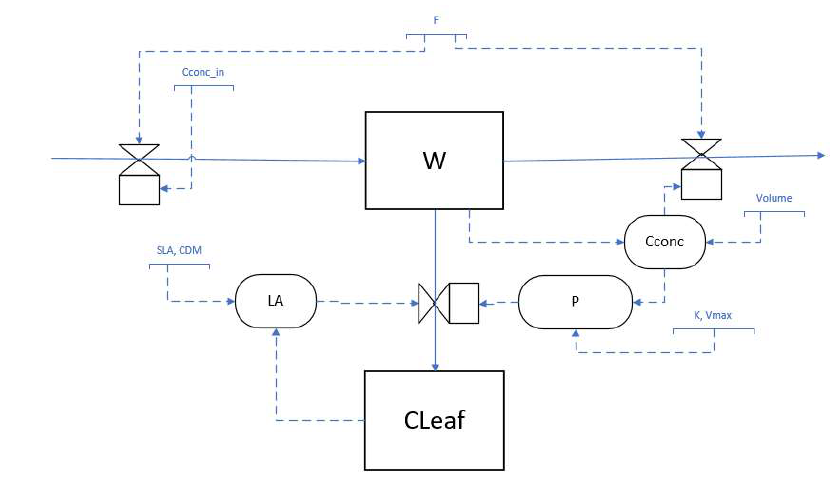
We continue with a model that calculates leaf photosynthesis rates in an open leaf chamber system (e.g. Exercise 5.2). We add the carbon in the leaf as part of the system and therefore reconsider the system boundaries. It makes sense to express all states in the amount of carbon, grams of . Note that this will also change the unit of in gC m-2 s-1.
The initial value for can be found from the following equation:
with the following units:
The initial value for (; amount of C in chamber) from the equation:
with the following units
To get in units, the same equation is used, but is replaced by the actual concentration in the chamber (thus at time step t).
Note that the parameter is
reflecting a constant that should not be changed by a user and
can therefore best be placed inside the body of the
ParmsCUVET2 function that defines parameter values.
CIN - COUT = W + CLeaf - (W0 + CLeaf0)
BAL(t) = W(t) + CLeaf(t) - (W0 + CLeaf0) - CIN(t) + COUT(t)
To check the mass balance, we now not only need to integrate the amount of C in the chamber and in the leafs, we now also need to keep track of all C that has entered the chamber (thus we need to integrate CIN), as well as all C that has left the chamber (we thus need to integrate also COUT). Hence, we now have two extra ‘state’ variables to make the mass balance check possible (CIN and COUT: they are not the real state variables were are interested in, but we need them for mass balance book-keeping).
Exercise 6.2
Implement the model
Looking back at the formulation of the questions and code of “CUVET1” and “CUVET2”, we were not very strict about the formulation of concentrations. Earlier we defined as the concentration of CO2 calculated by (gCO2 m-3), as is the amount of CO2. For consistency, you will add the newly formulated leaf growth dynamics (see 6.1) to the model, and change the basic state variable units from CO2 to C. Download therefore a template with the CUVET2 model (file CH6_CUVET2.r), which is our result version of exercise 5.2. In this exercise, by following the 5 steps below, you will adjust the model in order to account for the before mentioned changes and add mass a balance check:
- Step 1: Download the
CH6_CUVET2.r file. You will
adapt the rest of the model so that the leaf grows through the carbon
gain via photosynthesis. Since leaf growth is reflected by the increase
in leaf area, the parameter is no
longer needed. Instead, the area of the leaf has become an auxiliary
variable called . Create an equation
to calculate the leaf area () and add
the function to the
RatesCUVET2function. Make sure to adapt other parts of the function that use Area, so that they properly use of the variable. - Step 2: Add equations in the
ParamsCUVET2function to convert all parameters (, , ) that are expressed in gCO2 to a unit of gC using the parameter. Add units to the code (using#) to ensure that conversions are done properly. Note that should be placed inside theParamsCUVET2function, as this parameter is a constant that should not be changed by a user. - Step 3: To further complete the model, including
all aspects of exercise 6.1 a: add the state in the
InitCUVET2andRatesCUVET2function, and the parameters and for the carbon content per unit of dry matter of leaf in theParamsCUVET2function. Give a default value of 0.02 m2 g-1 and a default value of 0.45 g (C) g-1 (dry matter). - Step 4: In the
RatesCUVET2function, use the parameter to compute the concentration of CO2 in the chamber, and include this auxiliary variable to the output. Other auxiliary variables we want to output are and . - Step 5: Check if the model implementations are done
correctly. You can do so by doing a mass balance check, for which you
already defined the equation in exercise 6.1 c. Use the template that we
offer for adding mass balances, to understand how and where to add the
mass balance to your model! Add the different terms of the mass balance
equation to the correct location in the
MassBalanceCUVET2function provided in the file “CH6_CUVET2.r” that you have downloaded above. Ensure to check all units (yes, also in code) and if necessary, make the required conversions. Run the model for a period of 50 seconds with intervals of 1 second.
Step 1
The equation for LA (leaf area) equals:
The corresponding units are:
This has implications for the rate equation of CLeaf:
with the following units:
The adapted rate equation for W then becomes:
Step 2 + 3
A function returning the initial state values, and the starting values of the mass balance:
InitCUVET2 <- function(W = 0, CLeaf = 0){
  # Gather function arguments in a named vector
  y <- c(W     = W,      # g C in chamber
         CLeaf = CLeaf,  # g C in leaf biomass in chamber
         CIN   = 0,      # g C inflow, initial amount # this is included for the mass balance part of this exercise
         COUT  = 0)      # g C outflow, initial amount # this is included for the mass balance part of this exercise

  # Return the named vector
  return(y)
}
When the InitCUVET2 function is defined, the initial
conditions can be set using:
volume <- 0.0001 # m3
cini   <- 1.0    # initial CO2 concentration in g CO2 m-3
area   <- 0.01   # note that this is the Leaf Area (LA) at time 0
sla    <- 0.02   # m2 of leaf / g dry matter of biomass
cco2   <- 12 /44 # 12 g/mol for C, 44 g/mol for CO2.
cdm    <- 0.45   # gC g-1 dry matter of biomass

InitCUVET2(W = volume * cini * cco2,
           CLeaf = (area / sla) * cdm)
## W CLeaf CIN COUT
## 2.727273e-05 2.250000e-01 0.000000e+00 0.000000e+00Updated function definition of ParmsCUVET2, where
conversion from CO2 to C are done, and also with parameters and
are added. Note that the airflow (F in your forester diagram) is
indicated as ‘flow’ here in code. Likewise, the concentration of CO2 of
the airflow (Cconc_in in the Forester diagram) is indicated as ‘Cin’
here in code:
ParmsCUVET2 <- function(Volume = 0.0001,  # volume of the chamber, m3
                        flow   = 0.00001, # throughflow of air, m3/s
                        Cin    = 1.0,     # CO2 concentration of the inflowing air (g CO2 m-3)
                        Vm     = 0.001,   # Maximum rate of photosynthesis VM in g of CO2 m-2 s-1
                        K      = 1.0,     # K is the M-M constant of photosynthesis (g CO2 m-3)
                        SLA    = 0.02,    # m2 of leaf / g dry matter of biomass
                        CDM    = 0.45     # gC g-1 dry matter of biomass
                        ){
  # Constants
  CCO2 <- 12 /44 # 12 g/mol for C, 44 g/mol for CO2.

  # gC m-3 = gCO2 m-3 * gC/gCO2
  Cin <- Cin * CCO2

  # gC m-3 = gCO2 m-3 * gC/gCO2
  K <- K * CCO2

  # gC m-2 s-1 = gCO2 m-2 s-1 * gC/gCO2
  Vm <- Vm * CCO2

  # Gather function arguments in a named vector
  y <- c(CCO2 = CCO2,
         Volume = Volume,
         flow = flow,
         Cin = Cin,
         Vm = Vm,
         K = K,
         SLA = SLA,
         CDM = CDM)

  # Return named vector with values
  return(y)
}
Step 4 + 5
The function RatesCUVET2 can be updated to:
RatesCUVET2 <- function(t, y, parms) {
  with(as.list(c(y, parms)),{
    # Compute auxiliary/helper functions

    # Concentration of C inside the chamber
    # gC m-3 = gC / m-3
    C <- W / Volume

    # Concentration of C inside the chamber
    # gCO2 m-3 = gC * m-3 * gCO2/gC
    CO2 <- C / CCO2

    # Net rate of photosynthesis (no respiration assumed)
    # gC m-2(leaf) s-1
    P <- Vm * C / (C + K)

    # Calculate area of leaves from the biomass
    #m2 = gC * m2(leaf)/g DM * gDM gC-1
    LA <- CLeaf * SLA * 1 / CDM

    # Compute rate equations
    # gC s-1 = gC m-2 s-1 * m2
    dCLeafdt <- P * LA

    # gC s-1  =   m3 s-1 * gC m-3
    CIN <- flow * Cin # Inflow of C into the chamber
    COUT <- flow * C    # Outflow of C out of the  chamber

    # Net rate of change of amount of C in chamber
    # gC s-1 = gC s-1 - gC s-1 - gC s-1
    dWdt <- CIN - COUT - dCLeafdt

    # Gather all rates of change in a vector
    # - the rates should be in the same order as the states (as specified in 'y')
    # - it can be a named vector, but does not need to be
    RATES <- c(dWdt = dWdt,
               dCLeafdt = dCLeafdt)

    # Optional: get in/out flow used to compute mass balances (or set MB <- NULL)
    dCINdt <- CIN
    dCOUTdt <- COUT

    # Rates for balance terms, g of C s-1
    MB <- c(dCINdt = dCINdt,
            dCOUTdt = dCOUTdt)

    # Optional: gather auxiliary variables that should be returned (or set AUX <- NULL)
    # - this should be a named vector or list!
    AUX <- c(C = C,
             CO2 = CO2,
             P = P,
             LA = LA)

    # Return result as a list
    outList <- list(c(RATES, MB), # the rates of change
                    AUX) # additional output per time step
    return(outList)
  })
}
Mass balance in amounts of carbon:
and:
To implement in R, first define a function
MassBalanceCUVET2 that computes the mass balance for C:
MassBalanceCUVET2 <- function(y, ini, parms){
  # Add "0" to the state variables' names to indicate initial condition
  names(ini) = paste0(names(ini), "0")

  # As in the RatesCUVET2 function defined above, we can use the with() function to access elements directly by there name
  # here: 'y' is a deSolve matrix, so it is best to first convert it to a data.frame (using as.data.frame())
  # and then combine it with 'ini' using the function c()
  # and convert to a list using as.list()
  with(as.list(c(as.data.frame(y), ini, parms)), {
    # gC
    CBAL <-  ( W           # gC
              + CLeaf      # gC
              + COUT       # gC
              - W0         # gC, initial amount
              - CLeaf0     # gC, initial amount
              - CIN        # gC
              )

    return(CBAL)
  })
}
When the above is defined, the model can be solved using:
# Solve model
states <- ode(y = InitCUVET2(W = volume * cini * cco2,
                             CLeaf = (area / sla) * cdm),
              times = seq(from = 0, to = 50, by = 1),
              func = RatesCUVET2,
              parms = ParmsCUVET2(Volume = volume,
                                  SLA = sla,
                                  CDM = cdm),
              method = "ode45")
We can plot the model results:
plot(states)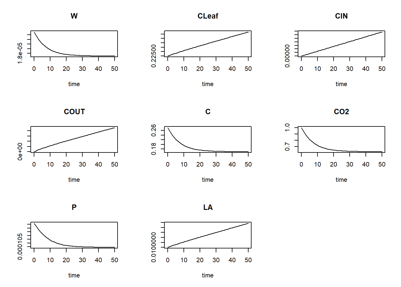
Lastly, and importantly, we can compute the mass balance:
# Compute mass balance
bal <- MassBalanceCUVET2(y = states,
                         ini = InitCUVET2(W = volume * cini * cco2,
                                          CLeaf = (area / sla) * cdm),
                         parms = ParmsCUVET2(Volume = volume,
                                             SLA = sla,
                                             CDM = cdm))

# Plot mass balance
par(mfrow=c(1,1)) # making sure the plot of the mass balance show up as a new image, instead of plotting it next to the model output.
plot(states[,"time"], bal,
     type = "l", xlab = "Time", ylab = "Mass balance, g C", col = "black")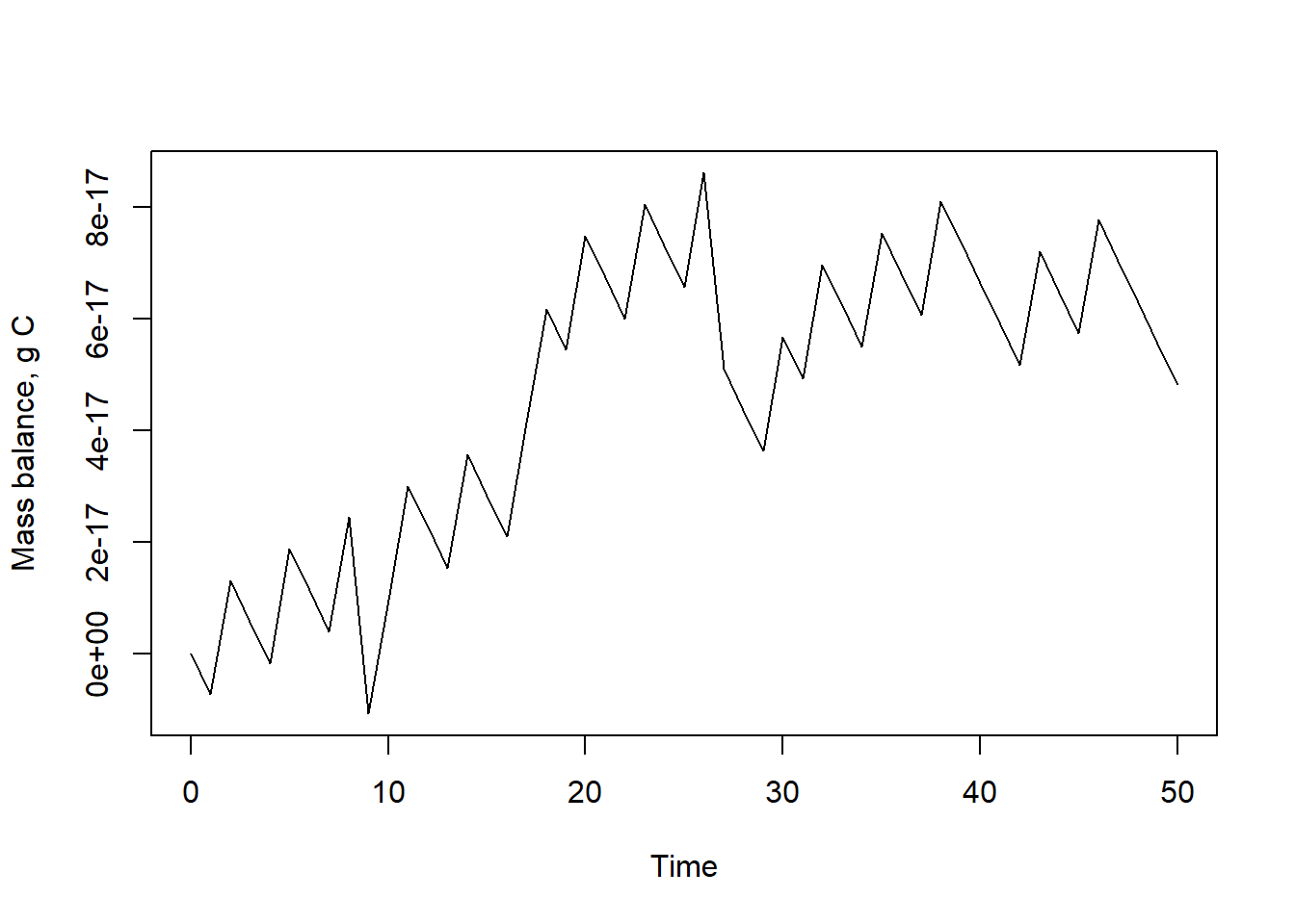
We see that the mass balance of C is very close to 0: carefully note
the y-axis values of the last plot: a value of -1e-16
actually means 0.0000000000000001, thus indeed very close to 0 (due to
numerical issues related to rounding and integration, it is
mathematically not exactly 0!).
In terms of modelled patterns and their interpretation: we see that CLeaf and LA are increasing over time, hence the leaf grows. Yet, we see that the amount of carbon in the chamber comes in equilibrium and so does leaf photosynthesis (P). In fact the model is rather unrealistic since it implies infinite leaf area growth.
Exercise 6.3
Do it now on your own!
Switching to another system, we will consider the decay of organic matter in a model that describes the total amount of organic carbon in a soil. This should be familiar to you from exercise 2.4. You will test the mass balance equation for this system.
A Forrester diagram is presented for dynamics in soil organic matter, with given names for state variables and parameters. There is only going into the system and going out of the system. All other parts of the rate equations detail internal flows and cancel out.
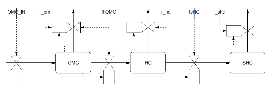
The balance can be calculated on-the go but also afterwards, which is done here in e.g. an auxiliary function. The following code produces the correct result with a balance nearly zero at all time steps, equivalent to 2000 years. Surprisingly, the error does change with parameter values (due to small rounding errors) but remains within the same order of magnitude. The increase in the error after a longer integration are due to the larger values for CIN and COUT, both increasing over time and containing large numbers. This can be understood when looking at the moment when errors start to increase. For larger values of R_OMC_IN this moment is reached earlier.
The implementation in R:
# A simple model to study SOC and OM decay
# See http://sites.biology.duke.edu/jackson/sbb2012.pdf
# for more models and parameters

# Define a function that returns a named vector with initial state values
InitOMDecay <- function(param) {
  # Initial conditions
  with(as.list(param),{
    # Amounts in kg per m-2 of soil
    IOMC <- (pOMC/100.) * SBD * DEPTH
    IHC  <- (pHC/100.) * SBD * DEPTH
    ISHC <- (pSHC/100.) * SBD * DEPTH

    # Gather in a named vector
    y <- c(OMC = IOMC, # kg m-2
           HC = IHC,   # kg m-2
           SHC = ISHC, # kg m-2
           IN = 0, OUT = 0) # for mass balance terms

    # Return named vector
    return(y)
  })
}

# Define a function that returns a named vector with parameter values
ParmsOMDecay <- function( # Set proportions of total SOM
  pOMC = 0.1,  # Normal SOM content is 4% so 2% SOC, for 1300 kg/m3 of mineral soil
  pHC = 1.6,
  pSHC = 0.3,
  SBD = 1300.0,# Soil bulk density, kg m-3
  DEPTH = 1.0, # soil depth, m
  # See e.g. Enriquez et al, 1993. r_om of 0.55 is a typical value
  r_om = 0.55, # r_om, relative turnover rate of OMC. Loss to atmosphere = r_om - fhOMC
  fhOMC = 0.1, # fraction of OMC annually turned over that becomes humus, y-1
  r_hc = 0.02, # typical rates for SOM breakdown around 2% p.a, or 2*2^((TAVG-9)/9), see Sattari et al 2014
  fsHC = 0.0005,
  r_shc = 0.005,
  # Plant litter: Decomposition, humus formation, carbon sequestration
  # about 0.5 kg / m2 / y is max based on 10000 kg DM/ha/y.
  R_OMC_IN =  0.15 # about 0.15 kg / m2 / y is needed to maintain SOC.
  ) {
  # Gather function arguments in a named vector
  y <- c(pOMC = pOMC, pHC = pHC, pSHC = pSHC, SBD = SBD, DEPTH = DEPTH,
           R_OMC_IN = R_OMC_IN,
           fhOMC = fhOMC, fsHC = fsHC,
           r_om = r_om, r_hc = r_hc, r_shc = r_shc)

  # Return the named vector
  return(y)
}

# Define a function for the rates of change of the state variables with respect to time
RatesOMDecay <- function(t, y, parms) {
  with(
    as.list(c(y, parms)),{

      # Rate equations, kg C m-2 y-1
      ROMC <- R_OMC_IN - (r_om - fhOMC) * OMC - fhOMC * OMC
      RHC  <- fhOMC * OMC - r_hc * HC  -  fsHC * HC
      RSHC <- fsHC * HC  - r_shc * SHC

      # Balance terms, kg C m-2
      RIN  <- R_OMC_IN             + fhOMC * OMC              + fsHC * HC
      ROUT <- (r_om - fhOMC) * OMC + fhOMC * OMC + r_hc * HC  + fsHC * HC + r_shc * SHC

      # Gather all rates of change in a vector
      # - the rates should be in the same order as the states (as specified in 'y')
      # - it can be a named vector, but does not need to be
      RATES <- c(ROMC=ROMC,
                 RHC = RHC,
                 RSHC = RSHC)

      # Get in/out flow used to compute mass balances
      MB <- c(RIN = RIN,
              ROUT = ROUT)

      # Optional: gather auxiliary variables that should be returned (or set AUX <- NULL)
      # - this should be a named vector or list!
      AUX <- NULL

      # Return result as a list
      # - the first element is a vector with the rates of change (in the same order as 'y')
      # - all other elements are (optional) extra output, which should be named
      outList <- list(c(RATES, MB), # the rates of change
                      AUX) # additional output per time step
      return(outList)
    }
  )
}

# Define a function to compute the mass balance over time
MassBalanceOMDecay <- function(y, ini) {
  # Add "0" to the state variables' names to indicate initial condition
  names(ini) = paste0(names(ini), "0")

  # Using the with() function we can access elements directly by there name
  # here: 'y' is a deSolve matrix
  # so it is best to first convert it to a data.frame using function as.data.frame()
  # and then combine it with 'ini' using the function c()
  # and convert to a list using as.list()
  with(as.list(c(as.data.frame(y), ini)), {
    BAL <- (OMC + HC + SHC) - (OMC0 + HC0 + SHC0) + OUT - IN
    return(BAL)
  })
}

# now we can solve the model and check mass balances over time
param <- ParmsOMDecay(R_OMC_IN = 0.15)
ini <- InitOMDecay(param)
states1 <- ode(y = ini,
               times = seq(0, 2000, by = 1),
               func = RatesOMDecay,
               parms = param,
               method = "ode45")
BAL1 <- MassBalanceOMDecay(y = states1, ini = ini)

param <- ParmsOMDecay(R_OMC_IN = 10)
ini <- InitOMDecay(param)
states2 <- ode(y = ini,
               times = seq(0, 2000, by = 1),
               func = RatesOMDecay,
               parms = param,
               method = "ode45")
BAL2 <- MassBalanceOMDecay(y = states2, ini = ini)

# Now we can plot it

plot(states1[,"time"], BAL1, type = "l", ylim = range(c(BAL1, BAL2)),
     xlab = "time", ylab = "C balance", col="black")
lines(states2[,"time"], BAL2, col="red",lty=2,lwd=2)
legend("topleft",legend=c("R_OMC_IN = 0.15","R_OMC_IN = 10"),
       col = c("black","red"), lty=c(1,1), lwd=c(1,2))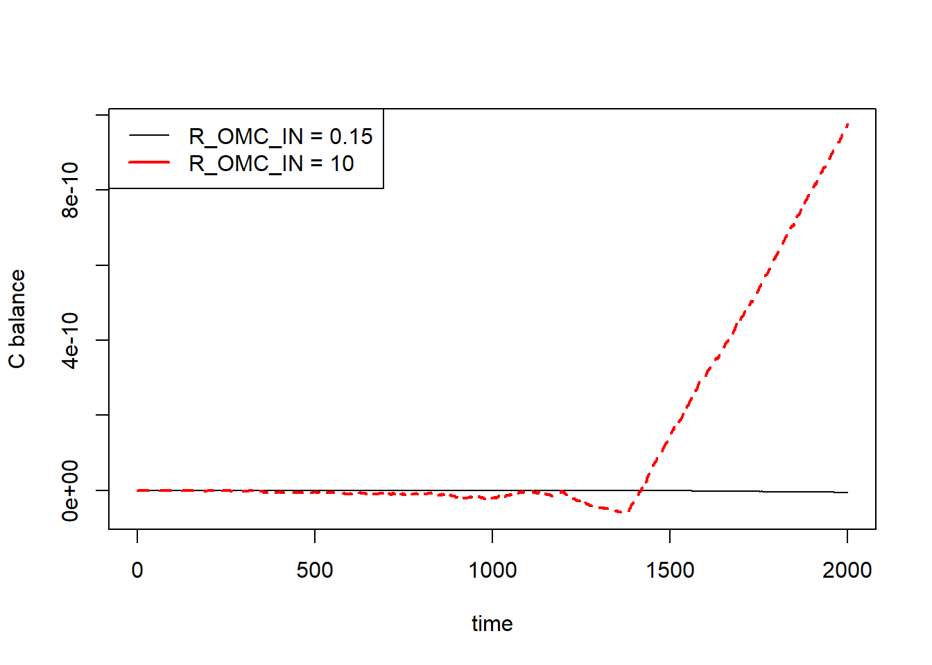
Exercise 6.4 (Optional)
For this exercise, once again we go back to the open leaf chamber
system, “CUVET2”. Evaluate the effect of parameters values on the
absolute error in the mass balance. Do this by changing the units for
and dry matter in 5 steps: from µg,
mg, g, kg and tonnes. This is most easily done by adding a parameter in the default
parameter list in the “parameter” function. This must have the following values
for the required conversions: 1e6 (for the conversion of g
to µg), 1e3 (g to mg), 1 (g to g), 1e-3 (g to
kg) or 1e-6 (g to ton). Ensure to use this parameter to change the values
of the parameters , , ,
and to the desired units as in this example
below. Explain why also the parameter value for needs to be adapted.
unit_factor <- 1e-6 # 1e3 from g to mg, 1e-6 from g to tonnes
# Convert units
Cini <- Cini * unit_factorWe will be comparing scenarios: with mass in ug, mg, g, kg and
tonnes, where an object UNIT_factor is defined, which
influences both initial state values and the value of some corresponding
parameters: all parameters that have a mass in the units (SLA, Cin, K,
Vm). We make sure that SLA is divided by the unit factor, as mass is in
the divider [m2 of leaf / g dry matter of biomass]. The other parameters
wer can convert by simply multiplying by the unit factor. Thus, we
update the ParmsCUVET2 function:
ParmsCUVET2 <- function(Volume = 1e-4,  # volume of the chamber, m3
                        flow   = 1e-5,  # throughflow of air, m3/s
                        Cin    = 1.0,   # CO2 concentration of the inflowing air (g CO2 m-3)
                        Vm     = 0.001, # Maximum rate of photosynthesis VM in g of CO2 m-2 s-1
                        K      = 1.0,   # K is the M-M constant of photosynthesis (g CO2 m-3)
                        SLA    = 0.02,  # m2 of leaf / g dry matter of biomass
                        CDM    = 0.45,  # gC g-1 dry matter of biomass
                        UNIT_factor = 1 # unit factor converting from g to mass unit of choice
                        ){
  # Constants
  CCO2 <- 12 /44 # 12 g/mol for C, 44 g/mol for CO2.

  # gC m-3 = gCO2 m-3 * gC/gCO2
  Cin <- Cin * CCO2 * UNIT_factor

  # gC m-3 = gCO2 m-3 * gC/gCO2
  K <- K * CCO2 * UNIT_factor

  # gC m-2 s-1 = gCO2 m-2 s-1 * gC/gCO2
  Vm <- Vm * CCO2 * UNIT_factor

  # SLA
  SLA <- SLA / UNIT_factor

  # Gather function arguments in a named vector
  y <- c(CCO2 = CCO2,
         Volume = Volume,
         flow = flow,
         Cin = Cin,
         Vm = Vm,
         K = K,
         SLA = SLA,
         CDM = CDM,
         UNIT_factor = UNIT_factor)

  # Return named vector with values
  return(y)
}
After updating ParmsCUVET2, we can now solve the model
for these scenarios and compute mass balance for each scenario:
# g to µg
unit_factor <- 1e6

# Solve the model
states_ug <- ode(y = InitCUVET2(W = volume * cini * cco2 * unit_factor,
                                CLeaf = (area / sla) * cdm * unit_factor),
                 times = seq(from = 0, to = 2000, by = 1),
                 func = RatesCUVET2,
                 parms = ParmsCUVET2(Volume = volume,
                                  SLA = sla,
                                  CDM = cdm,
                                  UNIT_factor = unit_factor),
                 method = "ode45")

# Compute the mass balance
bal_ug <- MassBalanceCUVET2(y = states_ug,
                            ini = InitCUVET2(W = volume * cini * cco2 * unit_factor,
                                             CLeaf = (area / sla) * cdm * unit_factor),
                            parms = ParmsCUVET2(Volume = volume,
                                                SLA = sla,
                                                CDM = cdm,
                                                UNIT_factor = unit_factor))

# g to mg
unit_factor <- 1e3

# Solve the model
states_mg <- ode(y = InitCUVET2(W = volume * cini * cco2 * unit_factor,
                                CLeaf = (area / sla) * cdm * unit_factor),
                 times = seq(from = 0, to = 2000, by = 1),
                 func = RatesCUVET2,
                 parms = ParmsCUVET2(Volume = volume,
                                  SLA = sla,
                                  CDM = cdm,
                                  UNIT_factor = unit_factor),
                 method = "ode45")
# Compute the mass balance
bal_mg <- MassBalanceCUVET2(y = states_mg,
                            ini = InitCUVET2(W = volume * cini * cco2 * unit_factor,
                                             CLeaf = (area / sla) * cdm * unit_factor),
                            parms = ParmsCUVET2(Volume = volume,
                                                SLA = sla,
                                                CDM = cdm,
                                                UNIT_factor = unit_factor))

# g to g
unit_factor <- 1

# Solve the model
states_g <- ode(y = InitCUVET2(W = volume * cini * cco2 * unit_factor,
                               CLeaf = (area / sla) * cdm * unit_factor),
                 times = seq(from = 0, to = 2000, by = 1),
                 func = RatesCUVET2,
                 parms = ParmsCUVET2(Volume = volume,
                                  SLA = sla,
                                  CDM = cdm,
                                  UNIT_factor = unit_factor),
                 method = "ode45")
# Compute the mass balance
bal_g <- MassBalanceCUVET2(y = states_g,
                           ini = InitCUVET2(W = volume * cini * cco2 * unit_factor,
                                            CLeaf = (area / sla) * cdm * unit_factor),
                           parms = ParmsCUVET2(Volume = volume,
                                                SLA = sla,
                                                CDM = cdm,
                                                UNIT_factor = unit_factor))

# g to kg
unit_factor <- 1e-3

# Solve the model
states_kg <- ode(y = InitCUVET2(W = volume * cini * cco2 * unit_factor,
                                CLeaf = (area / sla) * cdm * unit_factor),
                 times = seq(from = 0, to = 2000, by = 1),
                 func = RatesCUVET2,
                 parms = ParmsCUVET2(Volume = volume,
                                  SLA = sla,
                                  CDM = cdm,
                                  UNIT_factor = unit_factor),
                 method = "ode45")
# Compute the mass balance
bal_kg <- MassBalanceCUVET2(y = states_kg,
                           ini = InitCUVET2(W = volume * cini * cco2 * unit_factor,
                                            CLeaf = (area / sla) * cdm * unit_factor),
                           parms = ParmsCUVET2(Volume = volume,
                                                SLA = sla,
                                                CDM = cdm,
                                                UNIT_factor = unit_factor))


# g to ton
unit_factor <- 1e-6

# Solve the model
states_t <- ode(y = InitCUVET2(W = volume * cini * cco2 * unit_factor,
                               CLeaf = (area / sla) * cdm * unit_factor),
                 times = seq(from = 0, to = 2000, by = 1),
                 func = RatesCUVET2,
                 parms = ParmsCUVET2(Volume = volume,
                                  SLA = sla,
                                  CDM = cdm,
                                  UNIT_factor = unit_factor),
                 method = "ode45")
# Compute the mass balance
bal_t <- MassBalanceCUVET2(y = states_t,
                           ini = InitCUVET2(W = volume * cini * cco2 * unit_factor,
                                            CLeaf = (area / sla) * cdm * unit_factor),
                           parms = ParmsCUVET2(Volume = volume,
                                                SLA = sla,
                                                CDM = cdm,
                                                UNIT_factor = unit_factor))
Then, we can plot the results. We first plot the states W and CLeaf as function of time, for the first 50 seconds. To show that amounts are still the same, we convert all to g CO2 or gDM:
par(mfrow = c(1,2))

# Plot W as function of time, for all scenarios
plot(states_ug[,"time"], states_ug[,"W"] * 1e-6, main = "W", type = "l", lwd=2,
     xlim = c(0,50), xlab = "Time", ylab = "CO2 in chamber, g CO2",  col = "black")
points(states_mg[,"time"], states_mg[,"W"] * 1e-3, col = "blue", pch = 2)
points(states_g[,"time"], states_g[,"W"] * 1, col = "orange", pch = 2)
points(states_kg[,"time"], states_kg[,"W"] * 1e6, col = "red", pch = 3)
points(states_t[,"time"], states_t[,"W"] * 1e6, col = "green", pch = 4)

# Plot CLeaf as function of time, for all scenarios
plot(states_ug[,"time"], states_ug[,"CLeaf"] * 1e-6 , main = "CLeaf", type = "l", lwd=2,
     xlim = c(0,50), xlab = "Time",
     ylim = c(0.2250, 0.2251),
     ylab = "Biomass, g DM",  col = "black")
points(states_mg[,"time"], states_mg[,"CLeaf"] * 1e-3, col = "blue", pch = 2)
points(states_g[,"time"], states_g[,"CLeaf"] * 1, col = "orange", pch = 2)
points(states_kg[,"time"], states_kg[,"CLeaf"] * 1e6, col = "red", pch = 3)
points(states_t[,"time"], states_t[,"CLeaf"] * 1e6, col = "green", pch = 4)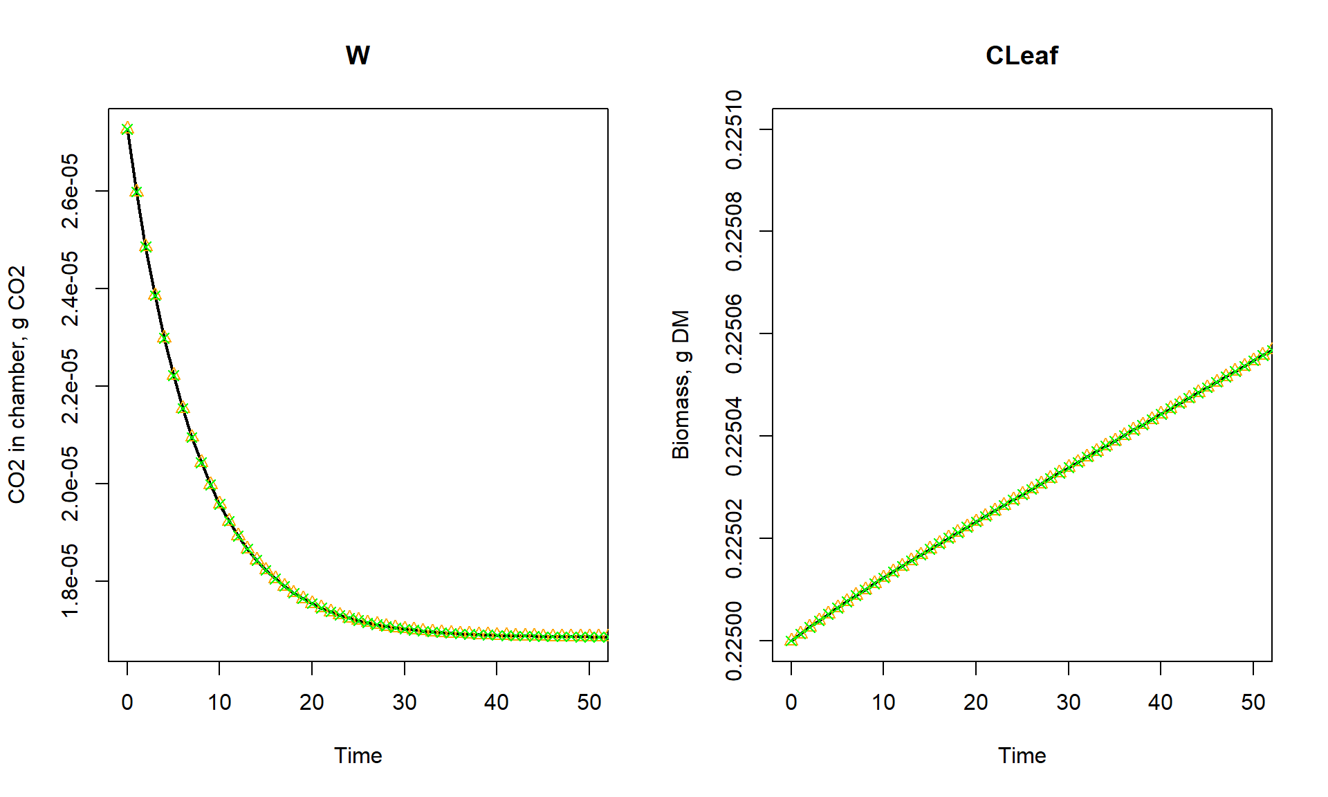
par(mfrow = c(1,1))The leaf grows steadily after an initial slow start due to CO2 shortage. We see that changing the units does not change the patterns of our modelled state variables (W and CLeaf)!
Let’s also plot the mass balances of the different scenarios:
par(mfrow = c(1,2))

# Absolute mass balances
plot(states_ug[,"time"], bal_ug, main = "Mass balance (absolute)", type = "l",
     xlim = c(0,2000), xlab = "Time",
     ylim = c(-1e-14, 1e-14), ylab = "Mass balance, g CO2", col = "black")
lines(states_mg[,"time"], bal_mg, col = "blue")
lines(states_g[,"time"], bal_g, col = "orange")
lines(states_kg[,"time"], bal_kg, col = "red" )
lines(states_t[,"time"], bal_t, col = "green" )

# Relative mass balances: dividing abolute mass balances by total amojunt
plot(states_ug[,"time"], bal_ug / (states_ug[,"W"] + states_ug[,"CLeaf"]),
     main = "Mass balance (relative)", type = "l",
     xlim = c(0,2000), xlab = "Time",
     ylim = c(-1e-14, 1e-14),
     ylab = "Mass balance, g CO2", col = "black")
lines(states_mg[,"time"], bal_mg / (states_mg[,"W"] + states_mg[,"CLeaf"]), col = "blue")
lines(states_g[,"time"], bal_g / (states_g[,"W"] + states_g[,"CLeaf"]), col = "orange")
lines(states_kg[,"time"], bal_kg / (states_kg[,"W"] + states_kg[,"CLeaf"]), col = "red" )
lines(states_t[,"time"], bal_t /(states_t[,"W"] + states_t[,"CLeaf"]), col = "green")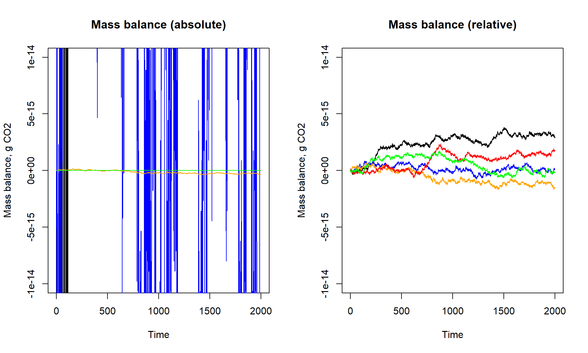
par(mfrow = c(1,1))The balance is around zero. The black line is for values computed in micrograms, blue in mg, orange in g, red in kg, green in tonnes; the lines shows the error (left plot: absolute, right plot: relative to total amoun tof C present) for each scenario.
Surprisingly, although we saw above that changing the units does not change the values of the state variables, changing the units does affect the balance error! Expressing units in kgg or tonnes, will store values in smaller decimal numbers and results in outcomes that are more precisely stored than for units in milli- or microgram. This is resulting from the lack of precision when storing these larger values, with single precision only whole integer values between -16777216 and 16777216 can be stored exactly. This can be easily seen when converting units to nanograms (factor 1e9), when the error even further increases when compared to micrograms. In other words, having a more precise unit requires more detailed information. When data are stored as smaller numbers (as units get larger), there is a rounding of information that works on all parameters similarly, reducing noise (small deviations) in calculations.
Solutions as R script
Download here the code as shown on this page in a separate .r file.