Wageningen University & Research | FEM-31806 | Models for Ecological Systems | FEM | PPS | WEC

Knowledge questions

Under what circumstances is numerical integration preferred over seeking an analytical solution, and what advantages does it offer in those situations?

Numerical integration is preferred when an analytical (closed‑form) solution is impossible, impractical, or inefficient to obtain.

This typically happens in situations such as:

The integrand is too complex so that an analytical solution is not possible (or even when a closed-form solution might exist in theory, it may be extremely complicated or computationally expensive to derive);
The integrand has irratic behaviour, such as sharp peaks, discontinuities (e.g. in the case of discrete event), or highly oscillatory behaviour. This makes analytical integration difficult, while numerical methods can adapt to these features;
The system includes a driving variable: external inputs (e.g. rainfall) often appear as arbitrary functions of time, and often are non-smooth and irregular, so that analytical integration becomes impossible.

Exercises

Have a look at the Templates section of this website, where we provide templates to solve ODE models using R. Following the naming convention used in the Templates, let’s call the function in this exercise “PredatorPrey”, thus below you will be defining the functions needed to conveniently solve the models and give them names like “InitPredatorPrey”, “ParmsPredatorPrey”, and “RatesPredatorPrey”.

In the syllabus and lecture, we were modelling the dynamics of a single population, but now we will be modelling a predator-prey system. The Lotka-Volterra model is a cornerstone for the theory about predator-prey interactions, and dates back to the 1920s. The basic Lotka-Volterra predator-prey model is based on the following assumptions:

prey would multiply indefinitely (i.e. grow exponentially) in the absence of predators;
predators would go extinct if prey were absent, due to a lack of food;
the proportional rate of increase of the prey decreases as the number of predators increases;
the growth rate of predators increases when the number of prey increases.

Using these assumptions, we can model the predator-prey system with a simple set of ordinary differential equations (ODE’s):

$\begin{aligned} \frac{dR}{dt} &= gR - bRC \\ \frac{dC}{dt} &= cbRC - mC \\ \end{aligned}$

where $R$ and $C$ represent the abundance of prey (Resource) and predators (Consumers), respectively. The parameter $g$ represents the exponential growth rate of prey in the absence of the predator, while $m$ represents the mortality rate of the predators in the absence of prey. Encounters between prey and predators are assumed to follow the mass action law and are hence proportional to the product of the abundances $R$ and $C$ . The parameter $b$ represents the attack/kill rate. The parameter $c$ represents the conversion efficiency, i.e. the efficiency with which predators convert consumed prey into biomass.

Exercise 4.1

Start RStudio and open a new script. Save the script at some convenient place. Load the package deSolve (install the package when it is not installed yet). In this exercise you are going to implement the predator-prey model as described above. Therefore, use the same names for the state variables ( $R$ and $C$ ) and the parameters ( $g$ , $b$ , $c$ , $m$ ), and call the rate variables that you will compute $dRdt$ and $dCdt$ . Information (and examples) that can be helpful are found in section 4.3 of the syllabus, as well as the template files provided on this website to solve ODE models numerically (for this exercise you can use Template 1).

4.1 a

Define a function that creates a named vector with the initial conditions for the state variables of the Lotka-Volterra predator-prey model. Name the function InitPredatorPrey, and specify the default values 0.5 for prey (or resource:

R

), and 0.1 for predator (or consumer:

C

InitPredatorPrey <- function(R = 0.5,  # Resource / prey
                             C = 0.1){ # Consumer / predator
  # Gather function arguments in a named vector
  y <- c(
    R = R,
    C = C
  )

  # Return the named vector
  return(y)
}

4.1 b

Define a function that creates a named vector with the parameters needed for the model. Name the function ParmsPredatorPrey, and set as default values: 0.5 for

g

, 1.0 for

b

, 0.5 for

c

and 0.1 for

m

ParmsPredatorPrey <- function(g = 0.5,  # exponential growth rate of prey in the absence of the predator
                              b = 1.0,  # attack/kill rate
                              c = 0.5,  # conversion efficiency
                              m = 0.1){ # mortality rate of the predators in the absence of prey
  # Gather function arguments in a named vector
  y <- c(
    g = g,
    b = b,
    c = c,
    m = m
  )

  # Return the named vector
  return(y)
}

4.1 c

Define a function, named RatesPredatorPrey, that computes the rates of change of the state parameters, and that will be evaluated by the ode() function. Remember that the ode() function requires the function to have as function arguments: t, y, parms (in that order, but you can use your own argument names, e.g. Time, State and Parms). Moreover, the function should return a list with as first element the rates of change of the state variables (here there are 2, so combine them in a vector using the function c()), in the order as specified in InitPredatorPrey.

RatesPredatorPrey <- function(t, y, parms) {
  # use the with() function to be able to access the parameters and states easily
  # remember that the with() function is with(data, expr), where
  # - 'data' is ideally a list with named elements
  #   thus: 'y' and 'parms' are combined using function c and converted using function as.list
  # - 'expr' is an expression (i.e. code) that is evaluated
  #   this can span multiple lines of code when embraced with curly brackets {}
  with(
    as.list(c(y, parms)), {
      # Optional: forcing functions: get value of the driving variables at time t (if any)

      # Optional: auxiliary equations

      # Rate equations
      dRdt <- g * R - b * R * C
      dCdt <- c * b * R * C - m * C

      # Gather all rates of change in a vector
      # - the rates should be in the same order as the states (as specified in 'y')
      # - it can be a named vector, but does not need to be
      RATES <- c(
        dRdt = dRdt,
        dCdt = dCdt
      )

      # Optional: get in/out flow used to compute mass balances (or set MB <- NULL)
      MB <- NULL

      # Optional: gather auxiliary variables that should be returned (or set AUX <- NULL)
      # - this should be a named vector or list!
      AUX <- NULL

      # Return result as a list
      # - the first element is a vector with the rates of change (in the same order as 'y')
      # - all other elements are (optional) extra output, which should be named
      outList <- list(
        c(
          RATES, # the rates of change of the state variables
          MB
        ), # the rates of change of the mass balance terms if MB is not NULL
        AUX
      ) # optional additional output per time step
      return(outList)
    }
  )
}

4.1 d

Specify a regular time series that starts at 0 and ends at 100 and increases with steps of 0.5, and assign it to a variable tseq. Use the function seq() for this.

tseq <- seq(from = 0, to = 100, by = 0.5)

4.1 e

Use the function ode() in the deSolve package to numerically solve the predator-prey model. Use the initial conditions (the function InitPredatorPrey created in (a)), parameter values (the function ParmsPredatorPrey as created in (b)) and function RatesPredatorPrey as created in (c). Use the variable tseq as input to the times argument in the call to the function ode(). Assign the solved ODE to the object states. Use “ode45” as the integration method supplied to method, i.e. an adaptive stepsize Runge-Kutta integration method (also in the following exercises when solving a model numerically).

states <- ode(
  y = InitPredatorPrey(),
  times = tseq,
  func = RatesPredatorPrey,
  parms = ParmsPredatorPrey(),
  method = "ode45"
)

4.1 f

Show the top and bottom rows of the object states (which essentially is a matrix) using the functions head() and tail(). What are the column names, and how do they relate to the initial state conditions as specified in InitPredatorPrey as created in exercise (a)?

head(states)

##      time         R         C
## [1,]  0.0 0.5000000 0.1000000
## [2,]  0.5 0.6093871 0.1092289
## [3,]  1.0 0.7385141 0.1229174
## [4,]  1.5 0.8875292 0.1432181
## [5,]  2.0 1.0533754 0.1735900
## [6,]  2.5 1.2269235 0.2195823

tail(states)

##         time            R         C
## [196,]  97.5 0.0014499409 0.8123317
## [197,]  98.0 0.0012526686 0.7729740
## [198,]  98.5 0.0011032233 0.7354916
## [199,]  99.0 0.0009895405 0.6998038
## [200,]  99.5 0.0009031619 0.6658312
## [201,] 100.0 0.0008380994 0.6334958

We can see that the columns names of the deSolve matrix states are “time” as well as “R” and “C”: the names of the states as specified in the input to argument y (the output of the function call InitPredatorPrey).

4.1 g

Plot the object states. Simply use plot(states) to use the default plot method for objects returned by the function ode.

plot(states)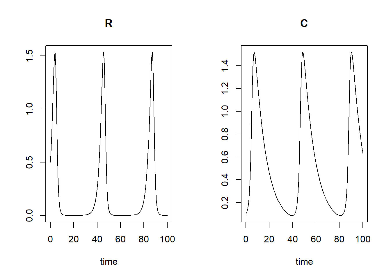

4.1 h

Plot

R

C

, with

R

on the x-axis and

C

on the y-axis. Note that the object states returned by the function ode() is a matrix. Also note that you’ve seen in (f) that the column names are “time”, “R” and “C” (the latter 2 because the function InitPredatorPrey specifies the 2 initial states to be “R” and “C”!). Remember that the column “R” can be retrieved using matrix indexing in different ways, here using either states[,2] or states[,"R"], because

R

is the second column, and has the column name “R”. A plot of x-values against y-values can be generated using plot(x = xvals, y = yvals, type = "l"), where xvals and yvals are hypothetical objects with data, and type = "l" specifies that the type of plot that is generated is a line plot. You can choose to adjust the axis labels by providing input to the arguments xlab and ylab.

plot(states[, "R"], states[, "C"], type = "l", xlab = "R", ylab = "C")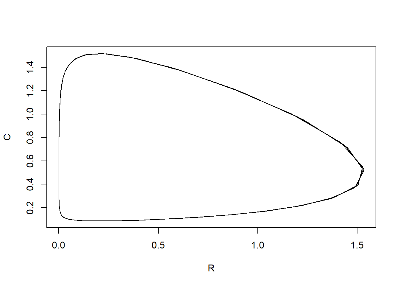

We see that when the resource increases, then also the consumer will increase, which will then cause a decrease in the resource, which will also result in a decrease in the consumer. This is a cycle that repeats itself over and over (the predator-prey cycle).

Note that the plotted line is not perfectly smooth: since we solve the model with time-steps of 0.5 (see how tseq was specified above); if we would solve the model with smaller a time-step, the line should look more smooth).

4.1 i

The nullclines (also called zero-growth isoclines) of the Lotka-Volterra predator-prey model are known: the nullcline $\frac{dR}{dt}=0$ is given $R=0$ and $C=\frac{g}{b}$ . The nullcline $\frac{dC}{dt}=0$ is given by $C=0$ and $R=\frac{m}{bc}$ . Obviously the nullclines where the states are 0 are not of interest (as we would not have a predator-prey system anymore). Thus, add the other 2 nullclines to the plot ( $C=\frac{g}{b}$ and $R = \frac{m}{bc}$ ). To do this, use the abline() function, where a line can be drawn horizontally or vertically at some value by specifying h=value or v=value, respectively. Alternatively, a linear line that is not parallel to the x or y axis can be drawn using the input arguments a=value and b=value, for intercept a and slope b. Use the same parameter values as passed to the function ode (thus retrieve these values from the ParmsPredatorPrey function).

Tip: it may be handy to use of the with function, and inside this the abline function:

with(as.list(ParmsPredatorPrey()), {
  abline(h = g / b, col = 8, lty = 2)
  abline(v = m / (b * c), col = 8, lty = 2)
})

plot(states[, "R"], states[, "C"], type = "l", xlab = "R", ylab = "C")

with(as.list(ParmsPredatorPrey()), {
  abline(h = g / b, col = 8, lty = 2)
  abline(v = m / (b * c), col = 8, lty = 2)
})

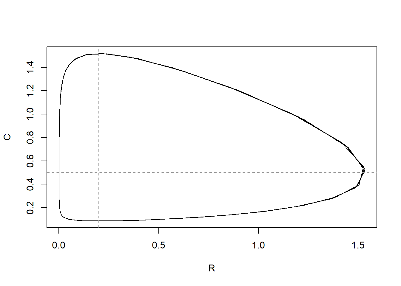
The nullclines indicate the situation where either the resource or the consumer does not change.

4.1 j

Solve the model for a longer duration: to 1000 time units, and assign it to a new object states2. Add the line of $R$ vs $C$ to the plot, using the function lines(). To specify the colour of the line, use the argument col (which can be a character string, e.g. “red” or “blue”, but also a value, e.g. 1 is black, 2 is red, 3 is green, etc). By adding the line in a different colour (than the current line in the plot), you can identify the added line easier.

Does solving the model for 1000 time units change the dynamics compared to solving it for 100 time units?

states2 <- ode(
  y = InitPredatorPrey(),
  times = seq(from = 0, to = 1000, by = 0.5),
  func = RatesPredatorPrey,
  parms = ParmsPredatorPrey(),
  method = "ode45"
)

plot(states[, "R"], states[, "C"], type = "l", xlab = "R", ylab = "C", col = "black")
lines(states2[, "R"], states2[, "C"], col = "red")

with(as.list(ParmsPredatorPrey()), {
  abline(h = g / b, col = 8, lty = 2)
  abline(v = m / (b * c), col = 8, lty = 2)
})

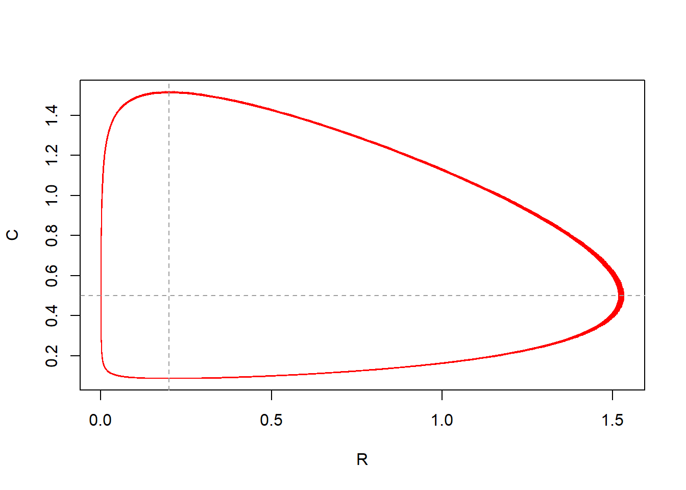
The output of the model solved for 1000 time units nicely fits the pattern as is already visible when solving the model for 100 time units. In the plot the added red line perfectly overlays the red line. Thus: solving the model for longer does not show different patterns; the predator-prey cycle pattern are already captured at 100 time units.

4.1 k

Add lines to the plot for 2 new scenarios: one where the initial conditions are

R=0.25

C=0.4

(save as states3), and one where the initial conditions are

R=0.2

C=0.45

(save as states4). For both scenarios, use the default parameter values and output times as specified in tseq. Add the lines with different colours so that you can identify the different scenarios. What can you conclude from the pattern shown in the plot? How does this match with the nullclines?

If we solve the model for different initial values of $R$ and $C$ we see that the result changes: the closer we initiate the states to the equilibrium, the smaller the cycles become:

plot(states[, "R"], states[, "C"], type = "l", xlab = "R", ylab = "C")

with(as.list(ParmsPredatorPrey()), {
  abline(h = g / b, col = 8, lty = 2)
  abline(v = m / (b * c), col = 8, lty = 2)
})

states2 <- ode(
  y = InitPredatorPrey(),
  times = seq(from = 0, to = 1000, by = 0.5),
  func = RatesPredatorPrey,
  parms = ParmsPredatorPrey(),
  method = "ode45"
)

lines(states2[, "R"], states2[, "C"], col = 2)

states3 <- ode(
  y = InitPredatorPrey(R = 0.25, C = 0.4),
  times = tseq,
  func = RatesPredatorPrey,
  parms = ParmsPredatorPrey(),
  method = "ode45"
)

lines(states3[, "R"], states3[, "C"], col = 4)

states4 <- ode(
  y = InitPredatorPrey(R = 0.2, C = 0.45),
  times = tseq,
  func = RatesPredatorPrey,
  parms = ParmsPredatorPrey(),
  method = "ode45"
)

lines(states4[, "R"], states4[, "C"], col = 3)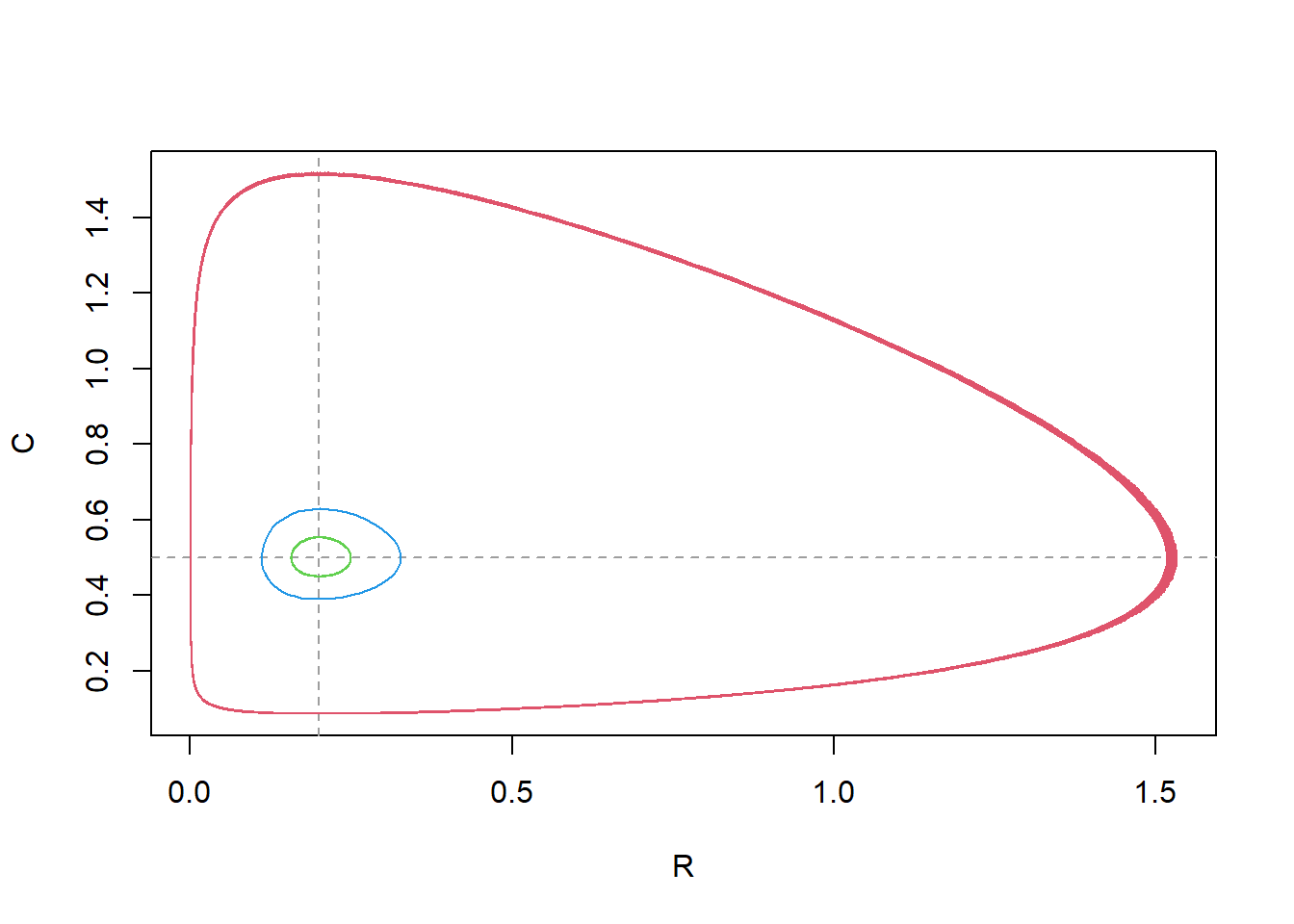

4.1 l

From the generated plot, and the nullclines as generated in (i), which initial conditions for the states will result in the absence of a cycle? Solve the set of ODEs for this set of initial conditions (and default parameter values, and output times as specified in tseq) and save as states5. Plot the solution.

When we first compute the equilibrium values of the states, and then initiate a simulation with those values, we see that the model stays in equilibrium throughout the simulation (what it is supposed to do):

stableInits <- with(as.list(ParmsPredatorPrey()), {
  c(R = m / (b * c), C = g / b)
})

states5 <- ode(
  y = stableInits,
  times = tseq,
  func = RatesPredatorPrey,
  parms = ParmsPredatorPrey(),
  method = "ode45"
)

plot(states5)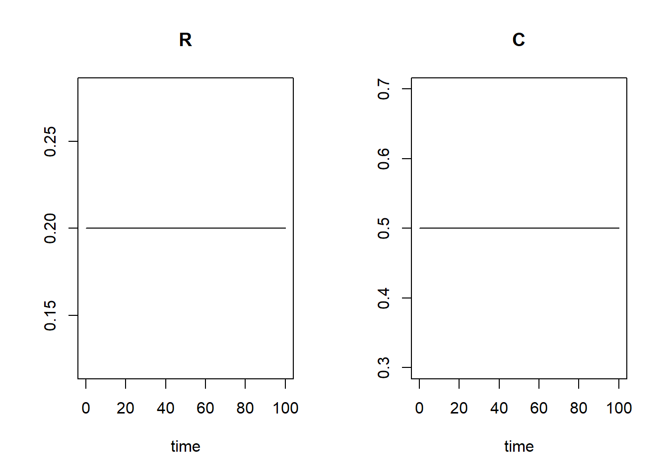

4.1 m

Plot states, states3, states4 and states5 in a single plot to compare the different scenarios (all evaluated on the same time scale tseq). Remember that the deSolve package allows for easy comparison of different scenarios by allowing multiple objects returned by the ode() function in a call to the plot() function, e.g. plot(states,states2).

We can plot multiple model simulations in a single plot:

plot(states, states3, states4, states5)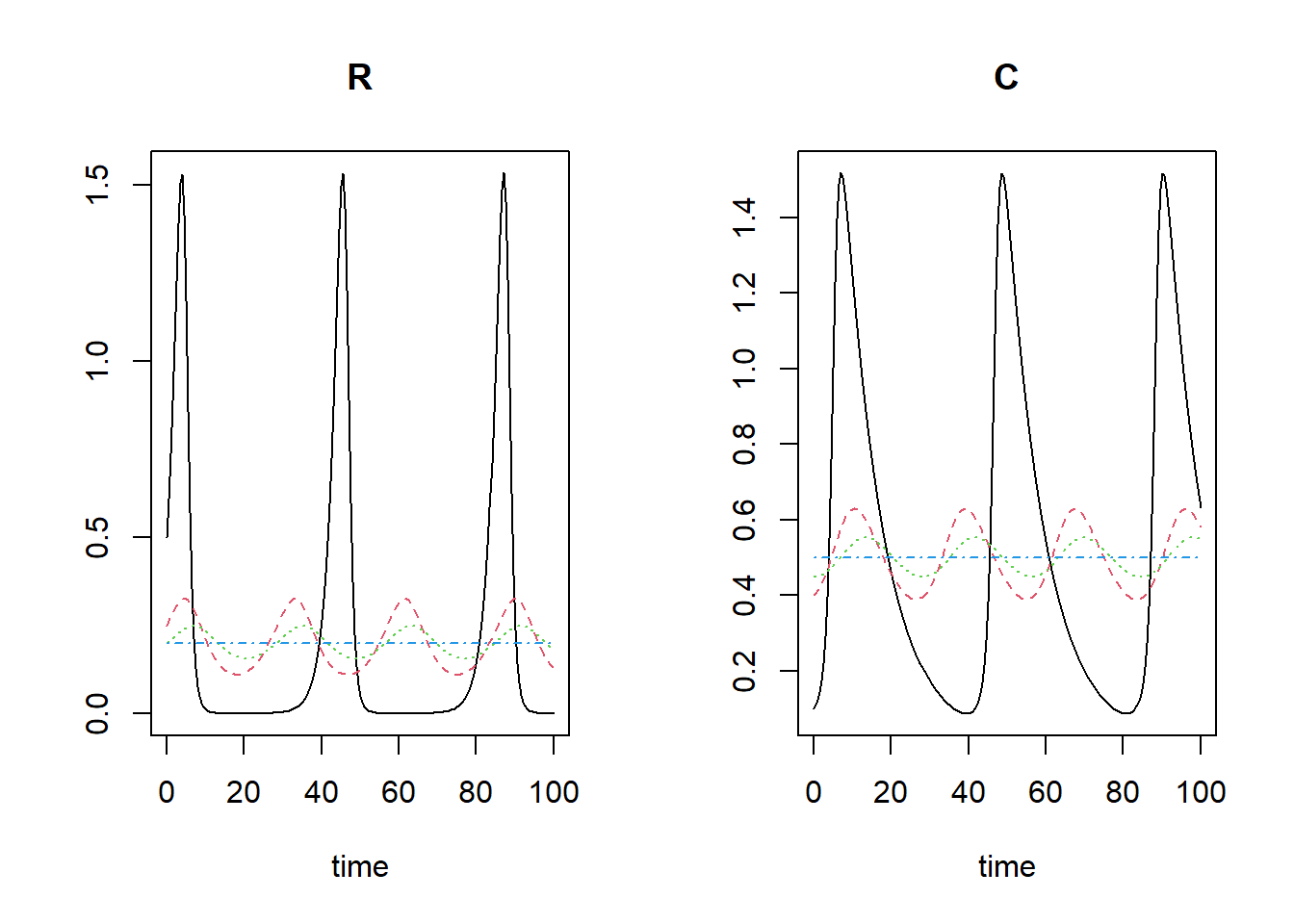

Note that the line colours and line-types follow the standard R colour/line-types 1:n, thus: the black line is for the first model, the red line is for the second model, the green line for model 3, blue for model 4.

Optional exercises

Exercise 4.2

A slightly more complicated and realistic version of the Lotka-Volterra predator-prey model assumes that prey do not grow indefinitely in the absence of predators but will ultimately reach a maximum prey abundance. Hence, prey do not grow exponentially, but follow, for example, a logistic growth equation, like we saw in the populations modelled in the syllabus and lectures. We can thus update the ODEs of the predator-prey model:

$\begin{aligned} \frac{dR}{dt} &= rR(1-\frac{R}{K}) - bRC \\ \frac{dC}{dt} &= cbRC - mC \\ \end{aligned}$

The only difference of this set of equations compared to the previous model is that we replaced the parameter $g$ with the term $r(1-\frac{R}{K})$ , characterizing the logistic growth process of prey up to a carrying capacity $K$ .

4.2 a

Create a new script that analyses this model including logistic growth for the prey. Copy parts from exercise 4.1 that you can re-use code (e.g. function InitPredatorPrey), whereas other parts (e.g. the functions ParmsPredatorPrey, and RatesPredatorPrey) should be updated (use the default values 0.5 for

r

and 10 for

K

). Give all functions now a new name, e.g. InitPredatorPrey2 etc. Solve the predator-prey system using the ode() function, using time-series stretching 100 time units (starting from 0 and ending at 100), but also longer (e.g. ending at 1000), and plot the results (both the default plot method, but also a plot with prey

R

on x-axis vs. predator

C

on y-axis). What is the main difference compared to the predator-prey system dynamics as seen in exercise 4.1?

InitPredatorPrey2 <- function(R = 0.5,  # Resource / prey
                              C = 0.1){ # Consumer / predator)
  # Gather function arguments in a named vector
  y <- c(
    R = R,
    C = C
  )

  # Return the named vector
  return(y)
}

ParmsPredatorPrey2 <- function(r = 0.5,  # intrinsic growth rate of logistic growth
                               K = 10,   # carrying capacity
                               b = 1.0,  # attack/kill rate
                               c = 0.5,  # conversion efficiency
                               m = 0.1){ # mortality rate of the predators in the absence of prey
  # Gather function arguments in a named vector
  y <- c(
    r = r,
    K = K,
    b = b,
    c = c,
    m = m
  )

  # Return the named vector
  return(y)
}

# Differences compared to exercise 4.1:
# - the rate equations
RatesPredatorPrey2 <- function(t, y, parms) {
  # use the with() function to be able to access the parameters and states easily
  # remember that the with() function is with(data, expr), where
  # - 'data' is ideally a list with named elements
  #   (thus combine 'y' and 'parms' first, using the function c(), then convert to list using as.list())
  # - 'expr' is an expression (i.e. code) that is evaluated
  #   this can span multiple lines of code when embraced with curly brackets {}
  with(
    as.list(c(y, parms)), {
      # Optional: forcing functions: get value of the driving variables at time t (if any)

      # Optional: auxiliary equations

      # Rate equations
      dRdt <- r * R * (1 - R / K) - b * R * C
      dCdt <- c * b * R * C - m * C

      # Gather all rates of change in a vector
      # - the rates should be in the same order as the states (as specified in 'y')
      # - it can be a named vector, but does not need to be
      RATES <- c(
        dRdt = dRdt,
        dCdt = dCdt
      )

      # Optional: get in/out flow used to compute mass balances (or set MB <- NULL)
      MB <- NULL

      # Optional: gather auxiliary variables that should be returned (or set AUX <- NULL)
      # - this should be a named vector or list!
      AUX <- NULL

      # Return result as a list
      # - the first element is a vector with the rates of change (in the same order as 'y')
      # - all other elements are (optional) extra output, which should be named
      outList <- list(
        c(RATES, MB), # the rates of change
        AUX
      ) # additional output per time step
      return(outList)
    }
  )
}

states <- ode(
  y = InitPredatorPrey2(),
  times = seq(from = 0, to = 1000, by = 0.5),
  func = RatesPredatorPrey2,
  parms = ParmsPredatorPrey2(),
  method = "ode45"
)

plot(states)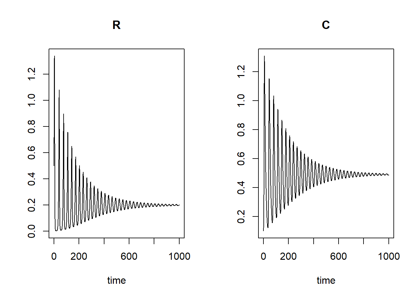

plot(states[, "R"], states[, "C"], type = "l", xlab = "R", ylab = "C")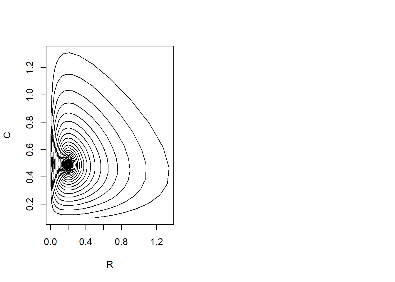

We can see that the main difference of the model from the previous exercises is that in this model the predator and prey will gradually oscillate to an equilibrium value: the cycles we saw in the previou exercises are getting smaller and smaller.

4.2 b

Compare different scenarios for the value of

K

. To do so, first create a vector

kseq

with 10 values ranging from 0.01 to 10 (the seq function is handy here). Then, create an empty list called outlist and iterate through the different scenarios (as specified in the vector kseq) using a for loop (see section 4.5 of the syllabus for examples, as well as section 3.11 for information on the use of loops). In each iteration i of the loop, use the i-th element of the vector kseq as the value for

K

, solve the ODE, and store the output in the i-th element of the list outlist (use double square brackets!). Then, plot the output using the plot method that deSolve offers for plotting multiple scenarios. Because you store all the scenarios in a single list, the following code will do the job: plot(outlist[[1]],outlist[-1]). This will create a plot with all scenarios.

kseq <- seq(from = 0.01, to = 10, length = 10)

outlist <- list()

for (i in 1:length(kseq)) {
  outlist[[i]] <- ode(
    y = InitPredatorPrey2(),
    times = seq(from = 0, to = 1000, by = 1),
    func = RatesPredatorPrey2,
    parms = ParmsPredatorPrey2(K = kseq[i]),
    method = "ode45"
  )
}

plot(outlist[[1]], outlist[-1])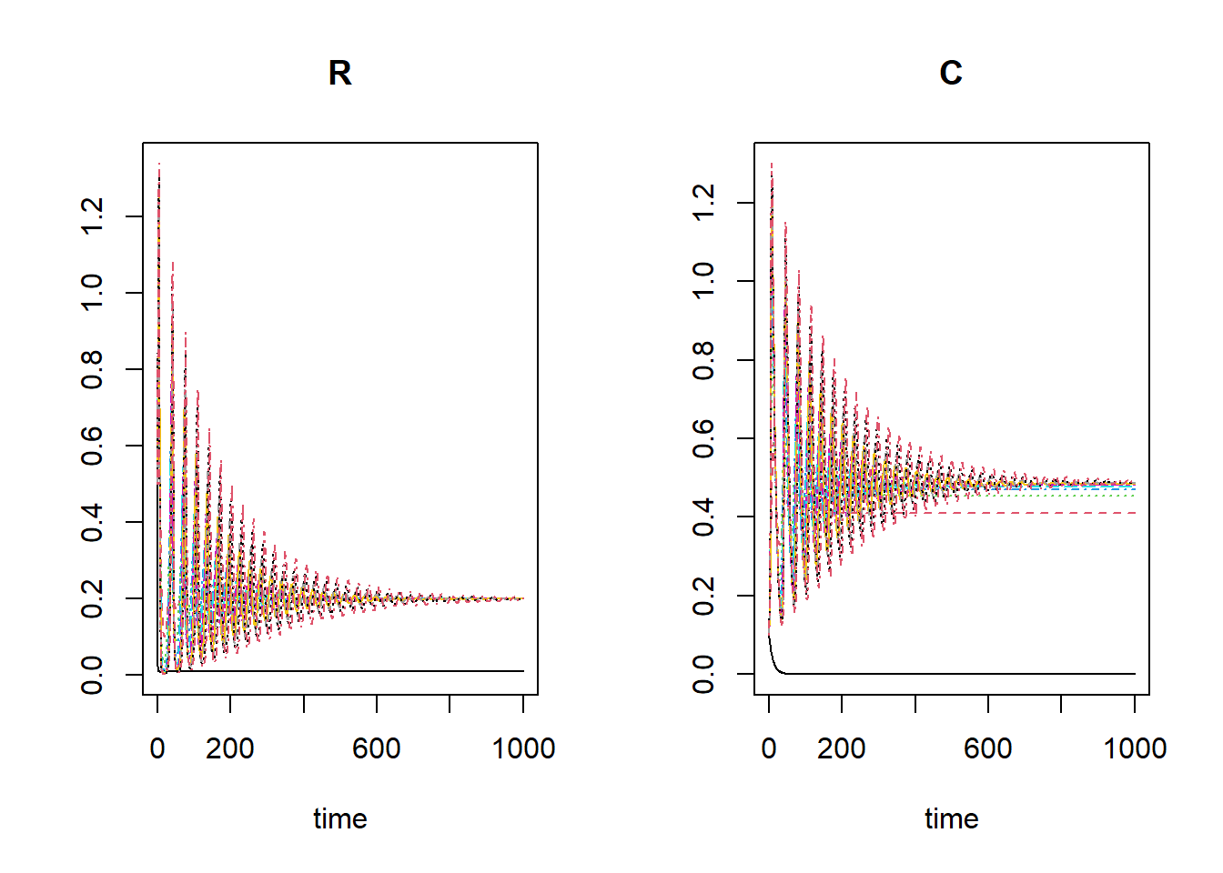

4.2 c

Repeat (b) but now with a sequence of

K

ranging from 0.01 to 1. Compare with the output of (b). What influence does the value of

K

have on the prey

R

, and what influence of predator

C

? Will there be a viable predator population in all scenarios?

kseq <- seq(from = 0.01, to = 1, length = 10)

outlist <- list()

for (i in 1:length(kseq)) {
  outlist[[i]] <- ode(
    y = InitPredatorPrey2(),
    times = seq(from = 0, to = 1000, by = 1),
    func = RatesPredatorPrey2,
    parms = ParmsPredatorPrey2(K = kseq[i]),
    method = "ode45"
  )
}

plot(outlist[[1]], outlist[-1])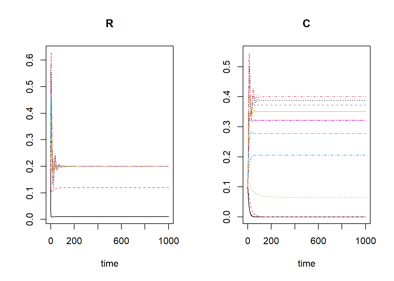

In most scenarios there will be a viable predator populaiton, yet in some scenarios the predator population will decrease to 0. This is the case for the ‘r nextinct’ lowest values of kseq: 0.01, 0.12.

Exercise 4.3

The models above assume that the attack/kill rate, $b$ , is constant and independent of $R$ and $C$ . However, this is often not realistic, e.g. when there is saturation in the need for food (e.g. as in the classical Rosenzweig-MacArthur predator-prey model), or when interference between predators reduces predation efficiency. Let’s assume that $b$ is not constant, but rather a function of $R$ and $C$ , as well as the parameters $b_1$ and $b_2$ :

$b = b_1 + b_2 \frac{R}{C}$

Everything else being equal, more predators will now lead to a lower attack efficiency. Do not bother too much with the ecological mechanism/realism of this equation: we now simply use it to practice skills for numerical integration!

4.3 a

Start a new script, and define a function attackRate using the formula above, with the default values 0.0 for

b_1

and 0.1 for

b_2

. Note that the values

b_1=1.0

and

b_2=0.0

result in a model that is actually the same as in the previous exercise! Plot the attack rate for R = 1:10, and C = c(0.25, 0.5, 1.0). Plot separate lines for the three values of

C

, in different colours so that you can easily identify the scenarios.

attackRate <- function(R, C, b1 = 0.0, b2 = 0.1) {
  y <- b1 + b2 * R / C
  return(y)
}

plot(1:10, attackRate(1:10, 0.25), type = "l", ylim = c(0, 5), xlab = "R", ylab = "attack rate")
lines(1:10, attackRate(1:10, 0.5), col = "red")
lines(1:10, attackRate(1:10, 1), col = "green")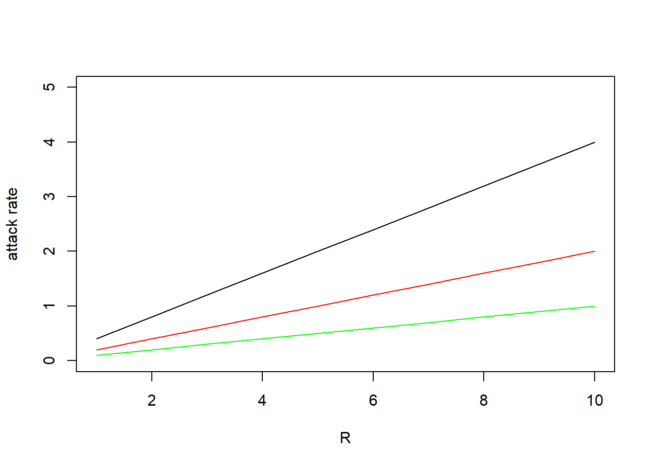

4.3 b

Copy/paste the InitPredatorPrey2, ParmsPredatorPrey2 and RatesPredatorPrey2 functions, and update where necessary! Give these functions the names InitPredatorPrey3 ParmsPredatorPrey3 and RatesPredatorPrey3 for this exercise. Note that the attack rate is used in 2 parts of the model: in the mortality of

R

, and in the growth or

C

. Thus, it may be most efficient to first compute the attack rate and assign it to an (auxiliary) variable, e.g. ar, and then use this variable in the rate equations. An advantage then is that you can choose to return the value of the auxiliary variable (remember: the first element of the list returned by RatesPredatorPrey3 contains the rate variables, so everything but the first element can be used to include auxiliary variables! See section 4.6 of the syllabus for examples).

InitPredatorPrey3 <- function(R = 0.5,  # Resource / prey
                              C = 0.1){ # Consumer / predator)
  # Gather function arguments in a named vector
  y <- c(
    R = R,
    C = C
  )

  # Return the named vector
  return(y)
}

ParmsPredatorPrey3 <- function(r = 0.5,  # intrinsic growth rate of logistic growth
                               K = 10,   # carrying capacity
                               b1 = 1.0, # attack/kill rate intercept
                               b2 = 0.0, # attack/kill rate slope
                               c = 0.5,  # conversion efficiency
                               m = 0.1){ # mortality rate of the predators in the absence of prey

  # Gather function arguments in a named vector
  y <- c(
    r = r,
    K = K,
    b1 = b1,
    b2 = b2,
    c = c,
    m = m
  )

  # Return the named vector
  return(y)
}

# Differences compared to exercise 4.2:
# - auxiliary function added
# - rate equations adjusted
# - 'ar' is returned as additional data
RatesPredatorPrey3 <- function(t, y, parms) {
  # use the with() function to be able to access the parameters and states easily
  # remember that the with() function is with(data, expr), where
  # - 'data' is ideally a list with named elements
  #   (thus combine 'y' and 'parms' first, using the function c(), then convert to list using as.list())
  # - 'expr' is an expression (i.e. code) that is evaluated
  #   this can span multiple lines of code when embraced with curly brackets {}
  with(
    as.list(c(y, parms)), {
      # Optional: forcing functions: get value of the driving variables at time t (if any)

      # Optional: auxiliary equations
      ar <- attackRate(R, C, b1, b2)

      # Rate equations
      dRdt <- r * R * (1 - R / K) - ar * R * C
      dCdt <- c * ar * R * C - m * C

      # Gather all rates of change in a vector
      # - the rates should be in the same order as the states (as specified in 'y')
      # - it can be a named vector, but does not need to be
      RATES <- c(
        dRdt = dRdt,
        dCdt = dCdt
      )

      # Optional: get in/out flow used to compute mass balances (or set MB <- NULL)
      MB <- NULL

      # Optional: gather auxiliary variables that should be returned (or set AUX <- NULL)
      # - this should be a named vector or list!
      AUX <- c(ar = ar)

      # Return result as a list
      # - the first element is a vector with the rates of change (in the same order as 'y')
      # - all other elements are (optional) extra output, which should be named
      outList <- list(
        c(RATES, MB), # the rates of change
        AUX
      ) # additional output per time step
      return(outList)
    }
  )
}
tseq <- seq(from = 0, to = 100, by = 1)

4.3 c

Solve the updated model for 3 scenarios:

b1=0.1, b2=0.0
b1=0.05, b2=0.05
b1=0.0, b2=0.01

which scenario is resulting in the highest predator density?

states1 <- ode(
  y = InitPredatorPrey3(),
  times = tseq,
  func = RatesPredatorPrey3,
  parms = ParmsPredatorPrey3(b1 = 0.1, b2 = 0.0),
  method = "ode45"
)

states2 <- ode(
  y = InitPredatorPrey3(),
  times = tseq,
  func = RatesPredatorPrey3,
  parms = ParmsPredatorPrey3(b1 = 0.05, b2 = 0.05),
  method = "ode45"
)

states3 <- ode(
  y = InitPredatorPrey3(),
  times = tseq,
  func = RatesPredatorPrey3,
  parms = ParmsPredatorPrey3(b1 = 0.0, b2 = 0.1),
  method = "ode45"
)

plot(states1, states2, states3)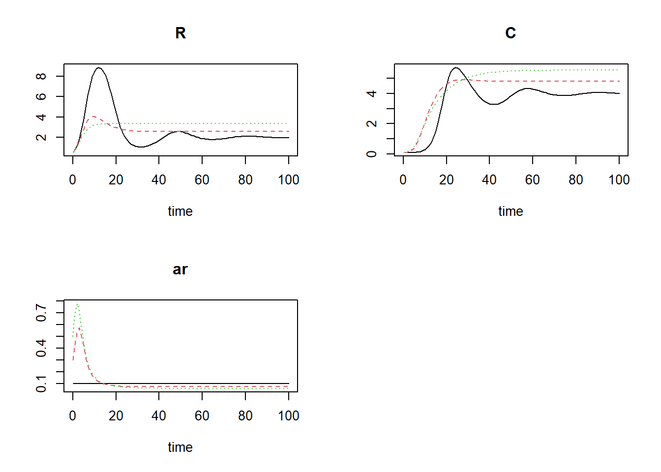

The third scenario (the green line in the plots) will ultimately result in the highest number of prey and predators (yet the attack rate will ultimately be the lowest).

Extra challenges

If you still have time, continue with the exercises below:

4.3 d

Try to find the value of parameter $b_2$ that maximizes the predator density $C$ , given the model above with $b_1=0.0$ . For this value of $b_2$ , what is the associated attack rate when the system is in balance (i.e. retrieve the value at the end of the integration, after verifying that the simulation has run long enough so that the system is in balance)?

Analyse a new scenario where you use this value (i.e. the associated attack rate) as the value for parameter

b_1

, where you set parameter

b_2=0.0

. How does the dynamics of this system differ from the one where

b_1=0.0

and

b_2

is set to the value maximizing the predator density?

# create empty list to store output data
outlist <- list()

# specify sequence of values for b2
b2seq <- seq(from = 1e-5, to = 0.1, length.out = 100)

# Iterate over all values of b2, solve model and store output
for(i in seq_along(b2seq)){
  outlist[[i]] <- ode(
    y = InitPredatorPrey3(R = 1, C = 0.1),
    times = seq(from = 0, to = 1000, by = 1),
    func = RatesPredatorPrey3,
    parms = ParmsPredatorPrey3(b1 = 0.0, b2 = b2seq[[i]]),
    method = "ode45"
  )
}

# Plot all simulations
plot(outlist[[1]], outlist[-1])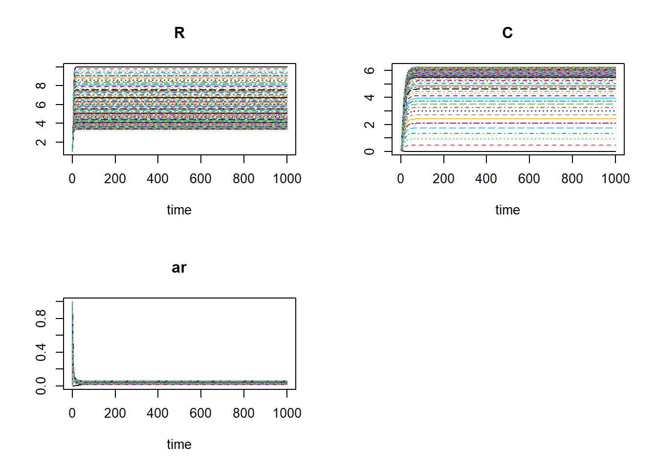

The system seems to have converged in all scenarios.

# Extract (state) values at final timestep
finalValues <- as.data.frame(
  do.call(
    rbind, 
    lapply(
      outlist, 
      function(x) {
        x[nrow(x), ]
      }
    )
  )
)
head(finalValues)

##   time        R           C       ar
## 1 1000 9.998000 0.004998001 0.020004
## 2 1000 9.800078 0.489811837 0.020408
## 3 1000 9.609840 0.937342695 0.020812
## 4 1000 9.426848 1.350754944 0.021216
## 5 1000 9.250694 1.732900550 0.021620
## 6 1000 9.081003 2.086354562 0.022024

# get value of b2 that maximizes the value for C
maxB2 <- b2seq[which.max(finalValues$C)]
maxB2

## [1] 0.0495

# Plot (with b2 value maximizing C indicated as vertical dashed line)
par(mfrow = c(2, 2))
plot(b2seq, finalValues$R, type = "l", xlab = "b", ylab = "R")
abline(v = maxB2, col = 8, lty = 2)
plot(b2seq, finalValues$C, type = "l", xlab = "b", ylab = "C")
abline(v = maxB2, col = 8, lty = 2)
plot(b2seq, finalValues$ar, type = "l", xlab = "b", ylab = "attack rate")
abline(v = maxB2, col = 8, lty = 2)
par(mfrow = c(1, 1))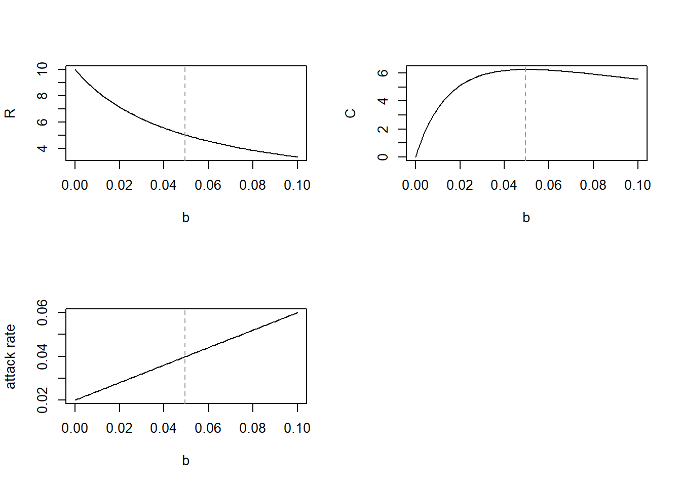

# What is the corresponding ar value at maximum C?
finalValues$ar[which.max(finalValues$C)]

## [1] 0.0398

# solve model with the b2 value that maximizes C (b1 = 0, b2 = 0.0495)
states1 <- ode(
  y = InitPredatorPrey3(R = 1, C = 0.01),
  times = seq(from = 0, to = 200, by = 1),
  func = RatesPredatorPrey3,
  parms = ParmsPredatorPrey3(b1 = 0.0, b2 = 0.0495),
  method = "ode45"
)

# solve model with corresponding ar value (b1 = 0.0398, b2 = 0)
states2 <- ode(
  y = InitPredatorPrey3(R = 1, C = 0.01),
  times = seq(from = 0, to = 200, by = 1),
  func = RatesPredatorPrey3,
  parms = ParmsPredatorPrey3(b1 = 0.0398, b2 = 0),
  method = "ode45"
)

# Plot both
plot(states1, states2)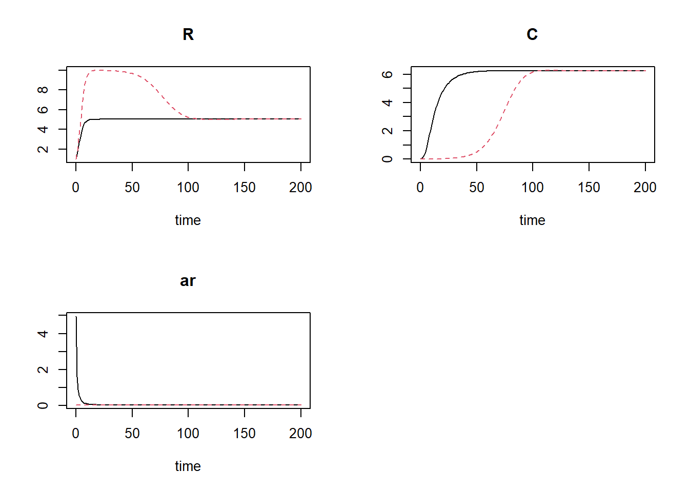

We see that now in both scenarios the system converges to the same equilibrium, yet with the model specification with parameter $b_2$ set to its optimum value (in terms of state $C$ ), the system converges much quicker.

4.3 e

Use the time series forcingK as created on page 94 of the syllabus, as well as the information on that page, to include

K

not as a constant, but a forcing function. Note: in the models in these exercises we’ve set

K

to 10, wereas the forcingK data is on average ca 100, thus divide the forcingK data (the column

K

) as retrieved from page 94 by 10 to have a time series that is variable yet on average equal to the value used in the previous exercises. The time series covers 50 time units, thus solve the ODE with

K

as a forcing function for 50 time units. Template 2 (on driving variables) can be of use here.

# data frame with info on driving variable
forcingK <- cbind(
  0:50,
  c(
    84, 82, 53, 67, 74, 123, 150, 136, 92, 105, 120, 136, 144, 117, 120, 136, 125,
    93, 108, 123, 113, 149, 112, 112, 51, 64, 109, 112, 98, 115, 90, 102, 65, 50,
    63, 66, 125, 150, 121, 120, 125, 120, 121, 139, 113, 96, 115, 82, 97, 101, 85
  )
)

# create forcing function
Kfun <- approxfun(x = forcingK[,1], y = forcingK[,2] / 10, method = "linear", rule = 2)

# update parameters function, remove K
ParmsPredatorPrey4 <- function(r = 0.5,  # intrinsic growth rate of logistic growth
                               b1 = 1.0, # attack/kill rate intercept
                               b2 = 0.0, # attack/kill rate slope
                               c = 0.5,  # conversion efficiency
                               m = 0.1){ # mortality rate of the predators in the absence of prey
  # Gather function arguments in a named vector
  y <- c(
    r = r,
    b1 = b1,
    b2 = b2,
    c = c,
    m = m
  )

  # Return the named vector
  return(y)
}

# update function with rate equations
# - difference with version 2 above: added forcing function and added as output to return list
RatesPredatorPrey4 <- function(t, y, parms) {
  # use the with() function to be able to access the parameters and states easily
  # remember that the with() function is with(data, expr), where
  # - 'data' is ideally a list with named elements
  #   (thus combine 'y' and 'parms' first, using the function c(), then convert to list using as.list())
  # - 'expr' is an expression (i.e. code) that is evaluated
  #   this can span multiple lines of code when embraced with curly brackets {}
  with(
    as.list(c(y, parms)), {
      # Optional: forcing functions: get value of the driving variables at time t (if any)
      K <- Kfun(t)

      # Optional: auxiliary equations
      ar <- attackRate(R, C, b1, b2)

      # Rate equations
      dRdt <- r * R * (1 - R / K) - ar * R * C
      dCdt <- c * ar * R * C - m * C

      # Gather all rates of change in a vector
      # - the rates should be in the same order as the states (as specified in 'y')
      # - it can be a named vector, but does not need to be
      RATES <- c(
        dRdt = dRdt,
        dCdt = dCdt
      )

      # Optional: get in/out flow used to compute mass balances (or set MB <- NULL)
      MB <- NULL

      # Optional: gather auxiliary variables that should be returned (or set AUX <- NULL)
      # - this should be a named vector or list!
      AUX <- c(
        ar = ar,
        K = K
      )

      # Return result as a list
      # - the first element is a vector with the rates of change (in the same order as 'y')
      # - all other elements are (optional) extra output, which should be named
      outList <- list(
        c(RATES, MB), # the rates of change
        AUX
      ) # additional output per time step
      return(outList)
    }
  )
}

# solve
states <- ode(
  y = InitPredatorPrey3(),
  times = seq(from = 0, to = 50, by = 0.1),
  func = RatesPredatorPrey4,
  parms = ParmsPredatorPrey4(),
  method = "ode45"
)

head(states)

##      time         R         C ar    K
## [1,]  0.0 0.5000000 0.1000000  1 8.40
## [2,]  0.1 0.5187882 0.1015588  1 8.38
## [3,]  0.2 0.5381300 0.1032402  1 8.36
## [4,]  0.3 0.5580257 0.1050525  1 8.34
## [5,]  0.4 0.5784735 0.1070044  1 8.32
## [6,]  0.5 0.5994695 0.1091056  1 8.30

plot(states)

4.3 f

Include also some discrete events: remove 25% of the prey population every 10 time units (at times 10,20,30 and 40). Solve the ODE with a forcing function (

K

) and events (harvesting prey) and plot the results. Template 3 (on discrete events) can be of use here.

# Define events
events <- list(data = data.frame(
  var = "R",
  time = c(10, 20, 30, 40),
  value = 0.75,
  method = "multiply"
))

# solve including events
states <- ode(
  y = InitPredatorPrey3(),
  times = seq(from = 0, to = 50, by = 0.1),
  func = RatesPredatorPrey4,
  parms = ParmsPredatorPrey4(),
  method = "ode45",
  events = events
)

# plot
plot(states)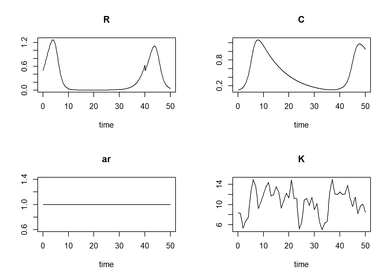

Solutions as R script

Download here the code as shown on this page in a separate .r file.

Chapter 4 - Numerical integration