# Set parameter values that influence the initial value of W
Volume <- 0.0001 # 0.1*10^-3 m3
Cini <- 10.0 # initial CO2 concentration in g CO2 m-3
# Solve model numerically with specified parameter values and variation in parameter K
states_ode45_K1 <- ode(
y = InitCUVET1(W = Volume * Cini),
times = seq(0, 2000, by = 1),
func = RatesCUVET1,
parms = ParmsCUVET1(K = 1,
Volume = Volume,
Cini = Cini), # all others at their default values
method = "ode45")
# Solve for other values of K
# ...
# Tips for plotting
# Plot dynamics of C as function of K:
plot(states_ode45_K10[, "time"], states_ode45_K10[, "C"],
type = "l", xlim = c(0, 200), ylim = c(0, 11),
xlab = "Time", ylab = "Conc. CO2", col = "black")
# tip to add lines to this graph, use the function lines()
# provide the x and y details in a similar fashion as in the plot() function
# If you want to save your plot, you can do this in many file types. Here is an example for storig your plot as pdf
# you first create a pdf using pdf(), then you write the code that creates your plot, and then you close the file with dev.off()
# As an example:
pdf("CUVET1_comparingKvalues.pdf") # name of the pdf file with the plot
plot(states_ode45_K1[,"time"], states_ode45_K1[,"W"],
type = "l", xlim = c(0,200), ylim = c(0,11),
xlab = "Time", ylab = "Amount of CO2", col = "black")
dev.off() # Close plotting devices
# The plot is saved to the working directory. Call getwd() to check!
# You can add as many things to the plot as you want:
# Once you call pdf() the file is created, and it only closes when dev.off() is runWageningen University & Research | FEM-31806 | Models for Ecological Systems | FEM | PPS | WEC
Chapter 5 - Equilibria, time-step and time coefficients
Knowledge questions
Consider the IJsselmeer lake (with an area of 1133 km2 and an average depth of 4.4 m, resulting in a volume of 4.532 km3) with inflow from the IJssel river (with a flow rate of 265 m3/s). The lake has a constant volume and hence inflow rates equal outflow rates. The change in the amount of pollutant in the lake can be described with the following differential equation:
Provide the time coefficient for this system.
Here the state is . The rate equation can be re-written as “something times ”:
When the inflow equals 0, the first part can be ignored. Then it is easy to see that the time coefficient for , , equals , or 1 divided by “what multiplies with the state”. This also looks like an negative exponential equation!
It can also be shown that this solution is correct with the general equation for the time coefficient and the equilibrium value for the state. The equilibrium value for :
When using this value in the equation for the time coefficient:
Note that this TC value is based on the assumption that the lake is perfectly mixed and that is only removed by outflow (so no decomposition or net precipitation on the lake floor).
Explain why the delay time is the same as the average residence time of
a pollutant .
This is an negative exponential system, most easy to see when inflow equals 0.
Explain what is meant by negative or positive feedbacks and indicate if
this system has no, a positive or a negative feedback.
A negative feedback means stability i.e. the system returns to the same equilibrium when a small change in the value of the state is made. A positive feedback is instable, and a small change will move the system away from an equilibrium. This system has a negative feedback. When the amount of is changed, it returns to the same equilibrium , equal to . This because the outflow rate increases when increases, so reducing the amounts in the lake, and the outflow rate decreases when decreased, increasing the amounts in the lake when the inflow remains unchanged.
Exercise 5.1
We can measure photosynthesis of a leaf or crop in a closed chamber by measuring the decrease in carbon dioxide concentration in time (like to the situation sketched in Exercise 2.1). The equation for the rate of change of the amount of carbon dioxide (, in g CO2) is given as:
where is the rate of photosynthesis in g CO2 m-2 s-1, and is the (single sided) surface area of a leaf or multiple leaves expressed in m2. is given by a so-called rectangular hyperbola:
where is the maximum rate of photosynthesis, and is the actual carbon dioxide concentration in the chamber, and is the concentration at which the rate of photosynthesis is half as large as the maximum.
The concentration is calculated from:
Where stands for the volume of the chamber. The parameters of the model are given as:
| Parameter | Unit |
|---|---|
| m3 | |
| m2 | |
| g CO2 m-2 s-1 | |
| g CO2 m-3 | |
| g CO2 m-3 |
Where is the initial CO2 concentration in the closed chamber.
5.1 a
Implement the above described model in R, in a script that you call
CUVET1.r. You can use the provided templates for that. Use
“CUVET1” as the model name (thus, define the functions
InitCUVET1, ParmsCUVET1, and
RatesCUVET1). The implementation of CUVET1:
# Define a function that returns a named vector with initial state values
InitCUVET1 <- function(W = 0){
  # Gather function arguments in a named vector
  y <- c(W = W)

  # Return the named vector
  return(y)
}

# Define a function that returns a named vector with parameter values
ParmsCUVET1 <- function(Volume = 0.0001, # volume of the chamber, m3
                        Area   = 0.01,   # area of leaves, m2
                        Vm   = 0.001,    # Maximum rate of photosynthesis VM in g of CO2 m-2 s-1
                        K      = 1.0,    # K is the M-M constant of photosynthesis
                                         # with respect to CO2 in same units as C
                        Cini   = 10.0){  # initial CO2 concentration in g CO2 m-3
  # Gather function arguments in a named vector
  y <- c(Volume = Volume,
         Area = Area,
         Vm = Vm,
         K = K,
         Cini = Cini)

  # Return named vector with values
  return(y)
}

# Define the function returning the rates of change of the state variables with respect to time
RatesCUVET1 <- function(t, y, parms){
  with(as.list(c(y, parms)),{
    # Compute auxiliary/helper functions

    # Concentration of CO2 inside the chamber
    C   <- W / Volume
    # Net rate of photosynthesis (no respiration assumed)
    P <- Vm * C / (K + C)

    # Compute rate equations

    # Net rate of change of amount of CO2 in chamber
    dWdt <- - P * Area

    # Gather all rates of change in a vector
    # - the rates should be in the same order as the states (as specified in 'y')
    # - it can be a named vector, but does not need to be
    RATES <- c(dWdt = dWdt)

    # Optional: get in/out flow used to compute mass balances (or set MB <- NULL)
    # not included here (thus here use MB <- NULL), see template 3
    MB <- NULL

    # Optional: gather auxiliary variables that should be returned (or set AUX <- NULL)
    # - this should be a named vector or list!
    AUX <- c(C = C, P = P)

    # Return result as a list
    # - the first element is a vector with the rates of change (in the same order as 'y')
    # - all other elements are (optional) extra output, which should be named
    outList <- list(c(RATES, MB), # the rates of change
                    AUX) # additional output per time step
    return(outList)
  })
}
5.1 b
Solve the implemented model numerically using the ode
function with values of 1, 10 and
0.1, and test if your model implementation works properly. The code
below gives a starting point for how to do this.
Above in the example code you find the ode function
call for a value of 1 (the restult of
which is stored to an object with name states_ode45_K1).
Evaluate this code and test if it works properly. Now model the change
in CO2 concentration over time with a value of 10 and 0.1. To do so, copy-paste
the ode function, change the name of the ode output (so that you don’t
store the new results over the previous model run), and adjust the values.
# Set parameter values that influence the initial value of W
Volume <- 0.0001  # 0.1*10^-3 m3
Cini   <- 10.0    # initial CO2 concentration in g CO2 m-3

# Solve model numerically with specified parameter values and variation in parameter K
states_ode45_K1 <- ode(
  y = InitCUVET1(W = Volume * Cini),
  times = seq(0, 2000, by = 1),
  func = RatesCUVET1,
  parms = ParmsCUVET1(K = 1,
                      Volume = Volume,
                      Cini = Cini), # all others at their default values
  method = "ode45")

states_ode45_K10 <- ode(
  y = InitCUVET1(W = Volume * Cini),
  times = seq(0, 2000, by = 1),
  func = RatesCUVET1,
  parms = ParmsCUVET1(K = 10,
                      Volume = Volume,
                      Cini = Cini), # all others at their default values
  method = "ode45")

states_ode45_K.1 <- ode(
  y = InitCUVET1(W = Volume * Cini),
  times = seq(0, 2000, by = 1),
  func = RatesCUVET1,
  parms = ParmsCUVET1(K = 0.1,
                      Volume = Volume,
                      Cini = Cini), # all others at their default values
  method = "ode45")

# Plot dynamics of C as function of K:
plot(states_ode45_K10[, "time"], states_ode45_K10[, "C"],
  type = "l", xlim = c(0, 200), ylim = c(0, 11),
  xlab = "Time", ylab = "Conc. CO2", col = "black")
lines(states_ode45_K1[, "time"], states_ode45_K1[, "C"], col = "blue")
lines(states_ode45_K.1[, "time"], states_ode45_K.1[, "C"], col = "red")

# add legend without a box
legend("topright", legend = c("K = 10", "K = 1", "K = 0.1"),
       col = c(" black", "blue", "red"), lty = c(1, 1, 1), bty = "n")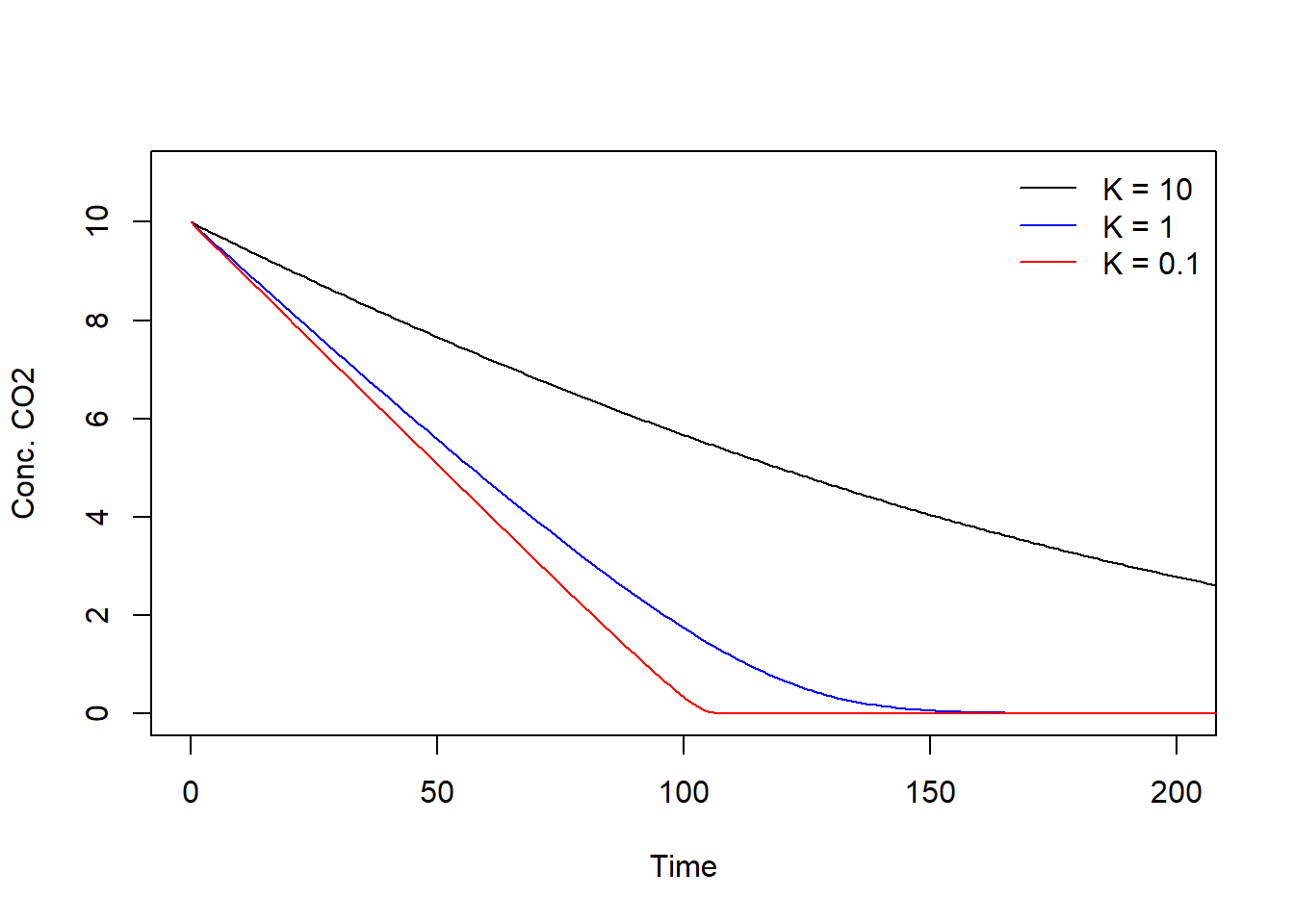
5.1 c
What are the consequences of a lower
value in terms of the photosynthetic rate of the leaf inside the
chamber? When is high (e.g. 10), photosynthesis is relatively slow which can be seen from the slow decrease in CO2 over time but also from the equation of ()– larger leads to a small value of , in turn leading to a smaller P. The smaller the K, the faster the photosynthesis which can be seen from the faster drop in CO2 over time but also from the equation of P – the closer gets to 0, the larger the value of , in turn leading to a larger .
5.1 d
Is it possible that the concentration in the chamber becomes negative?
Answer this question for the real system and speculate whether or when
for the model would return negative CO2 values. Negative concentrations are not physically possible. However, in the model it is possible! You may try this by setting the parameter to a negative value.
5.1 e
Let’s set to 0. What happens to the
specific photosynthetic rate of the leaf inside the chamber? Please give
your answer in relation to the equation for and describe in your own words what
happens. When K equals 0, K drops out of the ratio () in the photosynthesis equation, and this ratio becomes 1 since C is in both the numerator and denominator, making P independent of the CO2 concentration in the chamber. One exception exist, which is when C is 0, then the ratio cannot be determined and will produce an error due to the division by zero. In other words, the photosynthesis rate P equals the maximum rate of photosynthesis when .
5.1 f
Verify your answers by adding a new scenario to your code where . Add this result to your graph. Is this
the response you expected? Why (not)? states_ode45_K0 <- ode(
y = InitCUVET1(W = Volume * Cini),
times = seq(1, 2000, by = 1),
func = RatesCUVET1,
parms = ParmsCUVET1(Volume = Volume, Cini = Cini, K = 0),
method = "ode45"
)
plot(x = states_ode45_K1[, "time"], y = states_ode45_K1[, "C"],
type = "l", xlim = c(0, 200), ylim = c(0, 11),
xlab = "Time", ylab = "Conc. CO2", col = "blue")
lines(x = states_ode45_K10[, "time"], y =states_ode45_K10[, "C"], col = "black")
lines(x = states_ode45_K.1[, "time"], y =states_ode45_K.1[, "C"], col = "red")
lines(x = states_ode45_K0[, "time"], y =states_ode45_K0[, "C"], col = "green3")
# add legend without a box
legend("topright", legend = c("K = 10", "K = 1", "K = 0.1", "K = 0"),
col = c("black", "blue", "red", "green3"), lty = 1, bty = "n")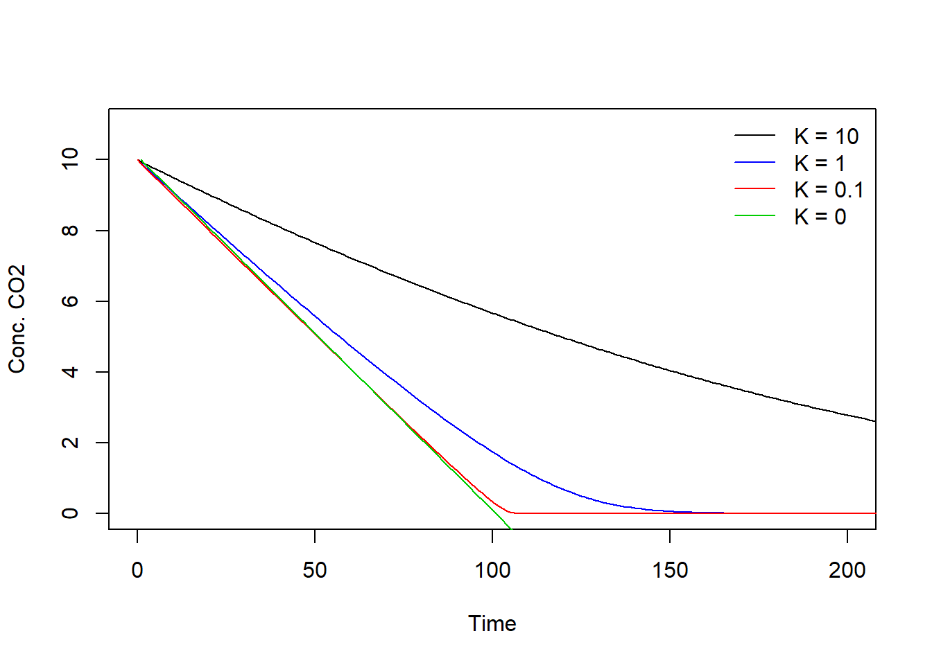
Exercise 5.2
As already explained in exercise 2.2, we measure leaf photosynthesis in a flow-through chamber. To this purpose the difference between the carbon dioxide concentration in the inflow and the outflow is measured in time. The rate of change of CO2 in the chamber becomes:
Here, is the concentration in the chamber and therefore also the CO2 concentration in the outflowing air. The new parameters of the model are set with the following default values:
- = 10.0 * 10-6 m3 s-1 (this can e set by the equipment)
- = 1.0 g CO2 m-3
- = 0.0 g CO2 m-3, which is the initial CO2 concentration in the chamber at t=0.
5.2 a
Copy the CUVET1.r file and rename it CUVET2.r. Change the model name to
CUVET2 and adapt the model accordingly. The implementation of CUVET2:
# Define a function that returns a named vector with initial state values
InitCUVET2 <- function(W = 0){
  # Gather function arguments in a named vector
  y <- c(W = W)

  # Return the named vector
  return(y)
}

# Define a function that returns a named vector with parameter values
ParmsCUVET2 <- function(Volume = 0.0001,  # volume of the chamber, m3
                        Area   = 0.01,    # area of leaves, m2
                        Flow   = 0.00001, # through flow of air, m3/s
                        Cin    = 1.0,     # CO2 concentration of the air flowing in (g CO2 m-3)
                        Vm     = 0.001,   # Maximum rate of photosynthesis VM in g of CO2 m-2 s-1
                        K      = 1.0,     # K is the M-M constant of photosynthesis
                                          # with respect to CO2 in same units as C
                        Cini   = 10.00){  # initial CO2 concentration in g CO2 m-3
  # Gather function arguments in a named vector
  y <- c(Volume = Volume,
         Area = Area,
         Flow = Flow,
         Cin = Cin,
         Vm = Vm,
         K = K,
         Cini = Cini)

  # Return named vector with values
  return(y)
}

# Define the function returning the rates of change of the state variables with respect to time
RatesCUVET2 <- function(t, y, parms){
  with(as.list(c(y, parms)),{
    # Compute auxiliary/helper functions

    # Concentration of CO2 inside the chamber
    C <- W / Volume
    # Net rate of photosynthesis (no respiration assumed)
    P <- Vm * C / (K + C)

    CIN  <- Cin * Flow # Inflow
    COUT <- C * Flow   # Outflow

    # Compute rate equations

    # Net rate of change of amount of CO2 in chamber
    dWdt <- CIN - COUT - P * Area

    # Gather all rates of change in a vector
    RATES <- c(dWdt)

    # Optional: get in/out flow used to compute mass balances (or set MB <- NULL)
    MB <- NULL

    # Optional: gather auxiliary variables (as named vector) that should be returned
    AUX <- c(C = C, P = P, CIN = CIN, COUT = COUT)

    # Return result as a list
    outList <- list(c(RATES, MB), # first element: the rates of change
                    AUX) # additional output per time step
    return(outList)
  })
}
5.2 b
Test whether the updated CUVET2 model runs, and solve the model for model for some different values, e.g. ; ; (for this see exercise 5.1b). Plot the restults in a plot like the one constructed in exercise 5.1b (thus: time on the x-axis, concentration CO2 on the y-axis, and separate lines for the separate values of K).
What are the implications of these values for the concentration in the chamber, and for leaf photosynthesis when concentrations become constant? Explain.Solving the model for different values of :
# Set parameter values that influence the initial value of W
Volume <- 0.0001 # m3
Cini   <- 0.0    # initial CO2 concentration in g CO2 m-3

# Solve model numerically with specified parameter values and variation in parameter K
states_ode45_K1 <- ode(
  y = InitCUVET2(W = Volume * Cini),
  times = seq(0, 200, by = 1),
  func = RatesCUVET2,
  parms = ParmsCUVET2(K = 1,
                      Volume = Volume,
                      Cini = Cini), # all others at their default values
  method = "ode45")

states_ode45_K10 <- ode(
  y = InitCUVET2(W = Volume * Cini),
  times = seq(0, 200, by = 1),
  func = RatesCUVET2,
  parms = ParmsCUVET2(K = 10,
                      Volume = Volume,
                      Cini = Cini), # all others at their default values),
  method = "ode45")

states_ode45_K.1 <- ode(
  y = InitCUVET2(W = Volume * Cini),
  times = seq(0, 200, by = 1),
  func = RatesCUVET2,
  parms = ParmsCUVET2(K = 0.1,
                      Volume = Volume,
                      Cini = Cini), # all others at their default values),
  method = "ode45")

# Plot dynamics of C as function of K:
plot(states_ode45_K10[, "time"], states_ode45_K10[, "C"],
  type = "l", xlim = c(0, 200), ylim = c(0, 1.2),
  xlab = "Time", ylab = "Conc. CO2", col = "black")
lines(states_ode45_K1[, "time"], states_ode45_K1[, "C"], col = "blue")
lines(states_ode45_K.1[, "time"], states_ode45_K.1[, "C"], col = "red")

# add legend without a box
legend("topright", legend = c("K = 10", "K = 1", "K = 0.1"),
       col = c(" black", "blue", "red"), lty = c(1, 1, 1), bty = "n")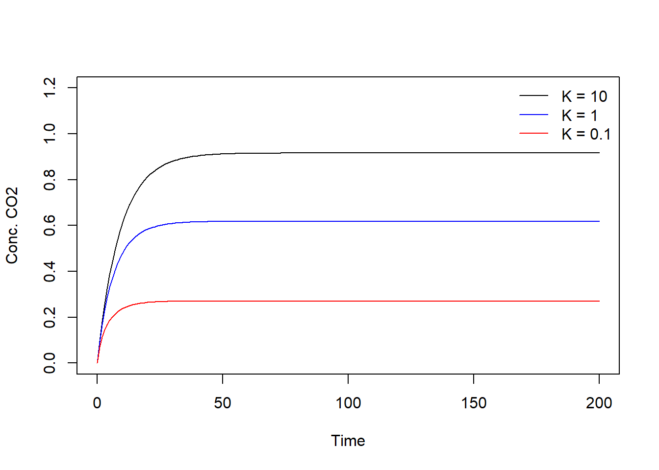
With a larger value, the photosynthetic rate becomes smaller, hence the uptake rate of CO2 from the air by the leaf in the chamber is smaller. When the system is in a (dynamic) equilibrium the resulting concentrations of CO2 will therefore be higher.
5.2 c
The expression for the dynamic equilibrium value of , i.e. the concentration, can be rewritten in the form of a quadratic function, which can be solved by the so-called “a-b-c” formula:
Derivation:
Set rate to zero and fill in the equations:
Multiply by (K+C) to eliminate C:
Eliminate parenthesis:
Divide by flow to simplify:
Re-arrange and combine terms:
This is a so-called quadratic function with the form , which can be solved with the abc-formula. Note that the variable (Capital!) (equilibrium C concentration) equals in the abc-formula, and that in the abc formula , , and .
Program the calculation of (make first a separate equation for , that simplifies a bit) in a separate function with the name “EquilCUVET2” that accepts the model parameters as argument. Then calculate the equilibria for the values 0.1, 1 and 10 (as done for question b) and add these to the corresponding plot using the lines function. Ensure to use argumentslty = 2 and lwd = 2 to display a thick dashed
line. Does your analytical solution for the equilibrium CO2
in the chamber indeed fit with the simulated dynamics? First, define a function (EquilCUVET2) that returns the
equilibria (given parameter values as input):
EquilCUVET2 <- function(param){
  with(as.list(param),{
    # algebraic solution of the steady state equation (C-equilibrium)
    B   <- K - Cin + Vm * Area / Flow
    CEQUIL <- -B/2.0 + sqrt((B/2.0)^2 + Cin * K)
    return(CEQUIL)
  })
}
Then, compute the equilibria for the K values 0.1, 1 and 10:
Volume <- 0.0001 # m3
Cini   <- 0.0      # initial CO2 concentration in g CO2 m-3
EqK0.1 <- EquilCUVET2(ParmsCUVET2(K = 0.1, Volume = Volume, Cini = Cini))
EqK1.0 <- EquilCUVET2(ParmsCUVET2(K = 1,   Volume = Volume, Cini = Cini))
EqK10  <- EquilCUVET2(ParmsCUVET2(K = 10,  Volume = Volume, Cini = Cini))
Lastly, plot the results
par(mfrow = c(2, 1), # 2 rows, 1 column
    mar = c(2, 4, 0.1, 0.1)) # with margins = c(bottom, left, top, right)

plot(states_ode45_K10[, "time"], states_ode45_K10[, "C"],
  type = "l", xlim = c(0, 50), ylim = c(0, 1.2),
  xlab = "Time", ylab = "Conc. CO2", lty = 1, lwd = 1, col = "black")
lines(c(-1E6, 1E6), c(EqK10, EqK10), lty = 2, lwd = 2, col = "black")
lines(states_ode45_K1[, "time"], states_ode45_K1[, "C"], lty = 1, lwd = 1, col = "blue")
lines(c(-1E6, 1E6), c(EqK1.0, EqK1.0), lty = 2, lwd = 2, col = "blue")
lines(states_ode45_K.1[, "time"], states_ode45_K.1[, "C"], lty = 1, lwd = 1, col = "red")
lines(c(-1E6, 1E6), c(EqK0.1, EqK0.1), lty = 2, lwd = 2, col = "red")

legend("topleft", legend = c("K=10", "K=1.0", "K=0.1"),
       col = c("black", "blue", "red"), lty = 1, bty = "n")

par(mar = c(4, 4, 0.1, 0.1))
plot(states_ode45_K10[, "time"], states_ode45_K10[, "P"],
  type = "l", xlim = c(0, 50), ylim = c(0, 8e-4),
  xlab = "Time", ylab = "Rate of photosynthesis", col = "black")
lines(states_ode45_K1[, "time"], states_ode45_K1[, "P"], col = "blue")
lines(states_ode45_K.1[, "time"], states_ode45_K.1[, "P"], col = "red")

legend("topleft", legend = c("K=10", "K=1.0", "K=0.1"),
       col = c("black", "blue", "red"), lty = 1, bty = "n")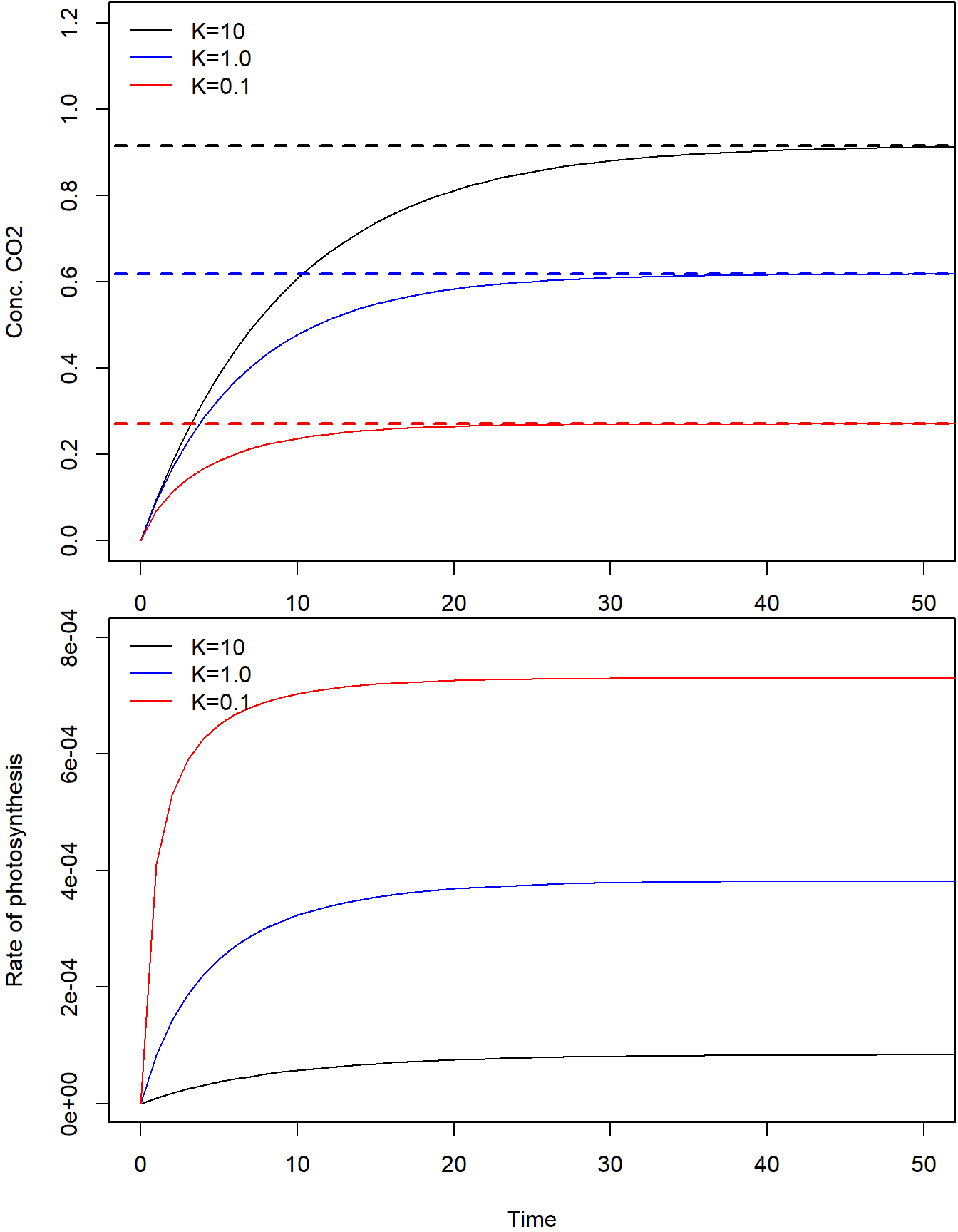
Eventually, the dynamic simulations result in the same equilibrium as the analytic result, providing confidence in the result. Note that the system reaches the equilibrium quicker when is 0.1 when compared to a of 10.
Exercise 5.3
What is the time coefficient for our system (see scripts developed for exercise 5.1) in a closed chamber? In this case, the equilibrium situation is achieved when the air in the cuvet does not contain anymore, i.e. .
5.3 a
First, estimate the time coefficient by assuming that specific
photosynthesis rates are equal to ,
irrespective of the amount of () in the chamber. The time coefficient of depletion can be estimated in various ways, depending on the precision of the definition. When assuming that the leaf photosynthesizes is equal to the maximum rate Vm all the time, irrespective of the CO2 concentration, we can estimate TC as follows: The initial amount of CO2 equals or 1 * 10-3 g. The rate of depletion then equals or 1 * 10-5 g s-1. The time to reach the equilibrium is then calculated from the ratio: TC = 100 s.
5.3 b
This approximation is incorrect since leaf specific photosynthesis rates
decreases when gradually becomes
lower in the leaf chamber. Therefore, find an analytical expression for
the time coefficient. Hint: this time
coefficient TC will change (with time) since it responds to a decrease
in . Rewrite the rate equation for
and express the equation
as function of . For this you need to
rework the equation to recognize the component that is multiplied with
. However, dW/dt is not constant and TC varies because decreases over time. To account for this, with , we rewrite dW/dt as a function of :
or
or
if we multiply by 1, or more precisely by VOLUME/VOLUME, we get:
since:
and thus:
where W cancels:
or,
Remarkably, the value of the time coefficient () decreases as W decreases, instead of being constant.
5.3 c
Once you have this equation, you can estimate the upper and lower limits
of TC. Hint: Do not use code yet but take a
good look at the equation and see how
and affect the TC. The upper asymptotic level for , so where is very small, is which is identical to our earlier calculation, because . The lower asymptotic limit for , so where has become very small, is . For the smallest value of (=0.1) this is equal to 1 second. We may conclude that, although the model is quite simple, the determination of the time coefficient of the model and the appropriate time step is not easy and depends on parameter values. This is especially important to know when we would use Euler as integration method.
5.3 d
Add the formula for the TC as an auxiliary variable to the
RatesCUVET1 function you have created above (exercise
5.1a). Ensure that you add this TC variable to the named list (as
auxiliary information) that is returned by the function.
Added parts to function RatesCUVET1 as already defined
above in exercise 5.1a):
# Compute the time coefficient
TC <- (W + K * Volume ) / (Area * Vm)

# Gather auxiliary information
AUX <- c(C = C, P = P, TC = TC)
Full function definition with these lines added:
# Define the function returning the rates of change of the state variables with respect to time
RatesCUVET1 <- function(t, y, parms){
  with(as.list(c(y, parms)),{
    # Compute auxiliary/helper functions

    # Concentration of CO2 inside the chamber
    C   <- W / Volume
    # Net rate of photosynthesis (no respiration assumed)
    P <- Vm * C / (K + C)

    # Compute rate equations

    # Net rate of change of amount of CO2 in chamber
    dWdt <- - P * Area

    # Gather all rates of change in a vector
    # - the rates should be in the same order as the states (as specified in 'y')
    # - it can be a named vector, but does not need to be
    RATES <- c(dWdt = dWdt)

    # Optional: get in/out flow used to compute mass balances (or set MB <- NULL)
    # not included here (thus here use MB <- NULL), see template 3
    MB <- NULL

    # Compute the time coefficient
    TC <- (W + K * Volume ) / (Area * Vm)

    # Optional: gather auxiliary variables that should be returned (or set AUX <- NULL)
    # - this should be a named vector or list!
    AUX <- c(C = C, P = P, TC = TC)

    # Return result as a list
    # - the first element is a vector with the rates of change (in the same order as 'y')
    # - all other elements are (optional) extra output, which should be named
    outList <- list(c(RATES, MB), # the rates of change
                    AUX) # additional output per time step
    return(outList)
  })
}
We can plot the TC after solving the model in the same way we did in exercise 5.1b):
Volume <- 0.0001 # m3
Cini   <- 10.0   # initial CO2 concentration in g CO2 m-3

states_ode45_K1 <- ode(
  y = InitCUVET1(W = Volume * Cini),
  times = seq(0, 2000, by = 1),
  func = RatesCUVET1,
  parms = ParmsCUVET1(K = 1,
                      Volume = Volume,
                      Cini = Cini), # all others at their default values
  method = "ode45")

states_ode45_K10 <- ode(
  y = InitCUVET1(W = Volume * Cini),
  times = seq(0, 2000, by = 1),
  func = RatesCUVET1,
  parms = ParmsCUVET1(K = 10,
                      Volume = Volume,
                      Cini = Cini), # all others at their default values
  method = "ode45")

states_ode45_K.1 <- ode(
  y = InitCUVET1(W = Volume * Cini),
  times = seq(0, 2000, by = 1),
  func = RatesCUVET1,
  parms = ParmsCUVET1(K = 0.1,
                      Volume = Volume,
                      Cini = Cini), # all others at their default values
  method = "ode45")
Now we can plot it:
par(mfrow = c(2, 2), mar = c(4, 4, 1, 1)) # with mar=c(bottom, left, top, right)

plot(states_ode45_K10[, "time"], states_ode45_K10[, "C"],
  type = "l", xlim = c(0, 200), ylim = c(0, Cini), xlab = "Time", ylab = "CO2, g/m3", col = "black")
lines(states_ode45_K1[, "time"], states_ode45_K1[, "C"], col = "blue")
lines(states_ode45_K.1[, "time"], states_ode45_K.1[, "C"], col = "red")

plot(states_ode45_K10[, "C"], states_ode45_K10[, "P"],
  type = "l", xlim = c(0, 10), ylim = c(0, 10E-4),
  xlab = "Conc. CO2", ylab = "Rate of photosynthesis", lty = 1, lwd = 1, col = "black")
lines(states_ode45_K1[, "C"], states_ode45_K1[, "P"], lty = 1, lwd = 1, col = "blue")
lines(states_ode45_K.1[, "C"], states_ode45_K.1[, "P"], lty = 1, lwd = 1, col = "red")

plot(states_ode45_K10[, "time"], states_ode45_K10[, "TC"],
  type = "l", xlim = c(0, 200), ylim = c(0, 200),
  xlab = "Time", ylab = "Time coefficient", lty = 1, lwd = 1, col = "black")
lines(states_ode45_K1[, "time"], states_ode45_K1[, "TC"], lty = 1, lwd = 1, col = "blue")
lines(states_ode45_K.1[, "time"], states_ode45_K.1[, "TC"], lty = 1, lwd = 1, col = "red")

# add legend without a box
legend("right", legend = c("K = 10", "K = 1", "K = 0.1"),
       col = c(" black", "blue", "red"), lty = c(1, 1, 1), bty = "n")

plot(states_ode45_K10[, "W"], states_ode45_K10[, "TC"],
  type = "l", xlim = c(0, Volume * Cini), ylim = c(0, 200),
  xlab = "W", ylab = "Time coefficient", lty = 1, lwd = 1, col = "black")
lines(states_ode45_K1[, "W"], states_ode45_K1[, "TC"], lty = 1, lwd = 1, col = "blue")
lines(states_ode45_K.1[, "W"], states_ode45_K.1[, "TC"], lty = 1, lwd = 1, col = "red")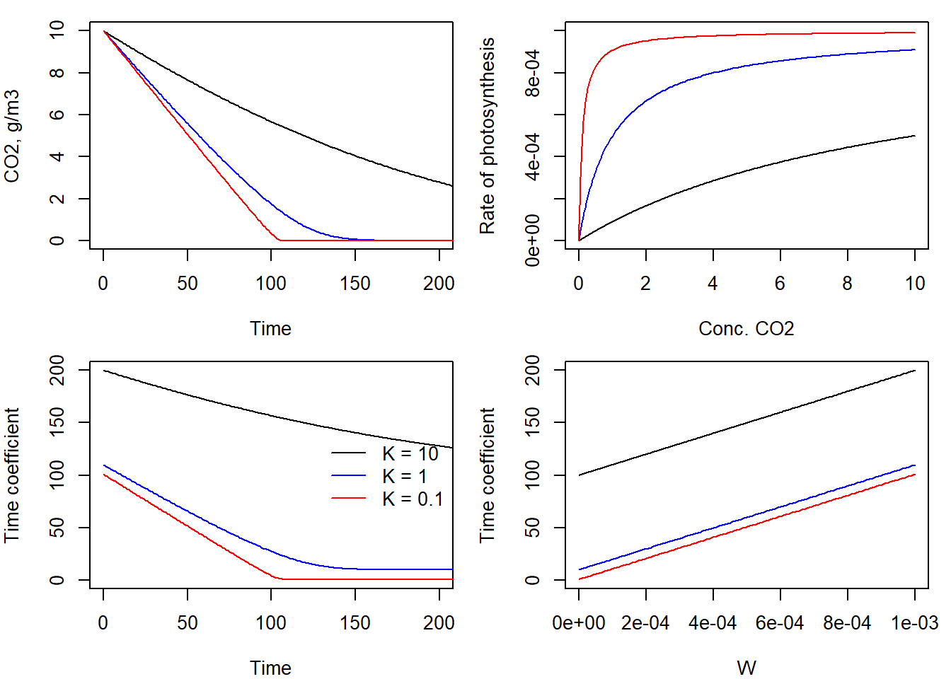
The plot of chamber concentration versus time, which shows a decreasing pattern with the abscissa (“x-axis”) as asymptote. The smaller the -value, the steeper the curve. For a very small value of , an almost linear decrease occurs until the CO2 is practically depleted. The plot of versus shows the three hyperbolic Michaelis-Menten relationships, as they evolve over the time of the simulation period. There is a numerical problem connected with the fact that numerically negative values of may occur, even though this is physically not possible. In the negative range of the hyperbolic relationship has a vertical asymptote at . For even more negative values of , the function value becomes positive again other “leg” of the hyperbola).
Solutions as R script
Download here the code as shown on this page in a separate .r file.