Wageningen University & Research | FEM-31806 | Models for Ecological Systems | FEM | PPS | WEC
Chapter 9 - Time step analysis
Knowledge questions
The numerical integration error must decrease when time steps taken are decreased. Time step convergence means that the model solution converges to the truth, i.e. the analytical solution when it is known. When this solution is not known, it can still be checked if the model follows the expectation that when time-steps are decreased by gradually smaller time steps, the solution should also show a gradual convergence to one solution where large time steps must result in large errors and small time steps in small errors.
A model with a fixed time-step of e.g. 1, takes steps of one time unit. When relevant parameters are expressed in absolute (or relative) value (or amount) per year, then also the rate equations will be expressed in an amount per year. Euler integration adds the rate times the time-step (of 1 year in this case) to the state: a time step of 1 therefore represents a step of one year and a constant rate of change during this whole year. This also means that if these relevant parameters are expressed in absolute (or relative) values (or amounts) per second, one time step will be one second as well and the rates of change will only be kept constant for a second. This solution is obviously more accurate!
Note that a variable time step will automatically adjust its time-step, so then changing parameter values from years to second may change the calculation time (as it may take more or less iterations to find an acceptable time step), but not the actual time steps taken by the model as these are defined by an acceptable integration error in the computed new value of the state.
Exercises
In the exercises you will use a mini-model with the name “ForSpace”
to study model behaviuor and test if model results converge when time
steps are changed using the time-base adjustment method. We will compare
the Euler with the Runge-Kutta integration. You will learn how you can
do a time-step analysis without changing the
time-step, but by expressing the parameter values that include a unit
time in another unit of time. The exercises for this chapter use the
ForSpace (mini) model, the code with the function definitions (with
functions InitForSpace, ParmsForSpace,
RatesForSpace and MassBalanceForSpace) can be
downloaded here. This
ForSpace model can be used to study the dynamics between two plant
species and two herbivore species.
Exercise 9.1
Download the R script
with the function definitions and save it to a convenient place (e.g. a
“scripts” folder in your working directory). Load the
deSolve package and run the downloaded script; either by
opening the file in R and running it, or by “sourcing” the script from
within the script file you are working in, e.g.:
# source script from file
source("scripts/CH9_ForSpace.r") # source the functions in this file into memory
Review the code of the ForSpace model (i.e. inspect the downloaded file). The unit of time is days.
Then, run the model using the example code and settings as shown below, and review the plots with the 4 state variables. Did the model reach equilibrium?
# Set AL1 here, to automatically change its value when used in the call to the ParmsForSpace function
setA11 <- 0.002 # 0.002 is the default

# Use deSolve to integrate derivatives numerically with Runge-Kutta and a variable time-step
states_ode45 <- ode(y = InitForSpace(),
                    time = seq(from = 0, to = 25000, by = 10),
                    func = RatesForSpace,
                    parms = ParmsForSpace(A11 = setA11),
                    method = "ode45")

# Define plotting settings
# Use the help function to understand what this function call using "par" does!
# Plot the states as function of time, with narrow plot margins.
par(mfrow = c(1,2), # nr of rows and columns, filled by row. defaults to c(1,1)
    mar = c(3, 3, 0.25, 0.25), # margins mar = c(bottom, left, top, right), default is c(5, 4, 4, 2) + 0.1
    mgp = c(1.5, 0.5, 0)) # margin line mgp = c(axes text, label, line) in mex units, default is c(3, 1, 0)

# Plot the  states to compare vegetation and herbivores
plot(states_ode45[,"time"], states_ode45[,"P1"], type = "l", col = "black",
     xlim = c(0,25000), ylim = c(0,700), xlab = "Time, d", ylab = "Plants, g biomass / m2")
lines(states_ode45[,"time"], states_ode45[,"P2"], type = "l", col = "red")
legend("topleft", lty = 1, col = c("black","red"), legend = c("P1","P2"), bty = "n")

plot(states_ode45[,"time"], states_ode45[,"H1"], type = "l", col = "black",
     xlim = c(0,25000), ylim = c(0,15), xlab = "Time, d", ylab = "Herbivores, g herbivore / m2")
lines(states_ode45[,"time"], states_ode45[,"H2"],type = "l",col = "red")
legend("topleft", lty = 1, col = c("black","red"), legend = c("H1","H2"), bty = "n")

# compute mass balance in grams
MBForSpace_ode45 <- MassBalanceForSpace(states_ode45,
                                        ini = InitForSpace(),
                                        parms = ParmsForSpace(A11 = setA11))

# plot mass balance balance after resetting plotting canvas
par(mfrow = c(1,1))
plot(MBForSpace_ode45[,"time"], MBForSpace_ode45[,"BAL"], type = "l", col = "black",
xlab = "Time, d", ylab = "Balance, g biomass/m2", ylim = c(-5e-10, 5e-10))# Set AL1 here, to automatically change its value when used in the call to the ParmsForSpace function
setA11 <- 0.002 # 0.002 is the default
# Use deSolve to integrate derivatives numerically with Runge-Kutta and a variable time-step
states_ode45 <- ode(y = InitForSpace(),
time = seq(from = 0, to = 25000, by = 10),
func = RatesForSpace,
parms = ParmsForSpace(A11 = setA11),
method = "ode45")
# Define plotting settings
# Use the help function to understand what this function call using "par" does!
# Plot the states as function of time, with narrow plot margins.
par(mfrow = c(1,2), # nr of rows and columns, filled by row. defaults to c(1,1)
mar = c(3, 3, 0.25, 0.25), # margins mar = c(bottom, left, top, right), default is c(5, 4, 4, 2) + 0.1
mgp = c(1.5, 0.5, 0)) # margin line mgp = c(axes text, label, line) in mex units, default is c(3, 1, 0)
# Plot the states to compare vegetation and herbivores
plot(states_ode45[,"time"], states_ode45[,"P1"], type = "l", col = "black",
xlim = c(0,25000), ylim = c(0,700), xlab = "Time, d", ylab = "Plants, g biomass / m2")
lines(states_ode45[,"time"], states_ode45[,"P2"], type = "l", col = "red")
legend("topleft", lty = 1, col = c("black","red"), legend = c("P1","P2"), bty = "n")
plot(states_ode45[,"time"], states_ode45[,"H1"], type = "l", col = "black",
xlim = c(0,25000), ylim = c(0,15), xlab = "Time, d", ylab = "Herbivores, g herbivore / m2")
lines(states_ode45[,"time"], states_ode45[,"H2"],type = "l",col = "red")
legend("topleft", lty = 1, col = c("black","red"), legend = c("H1","H2"), bty = "n")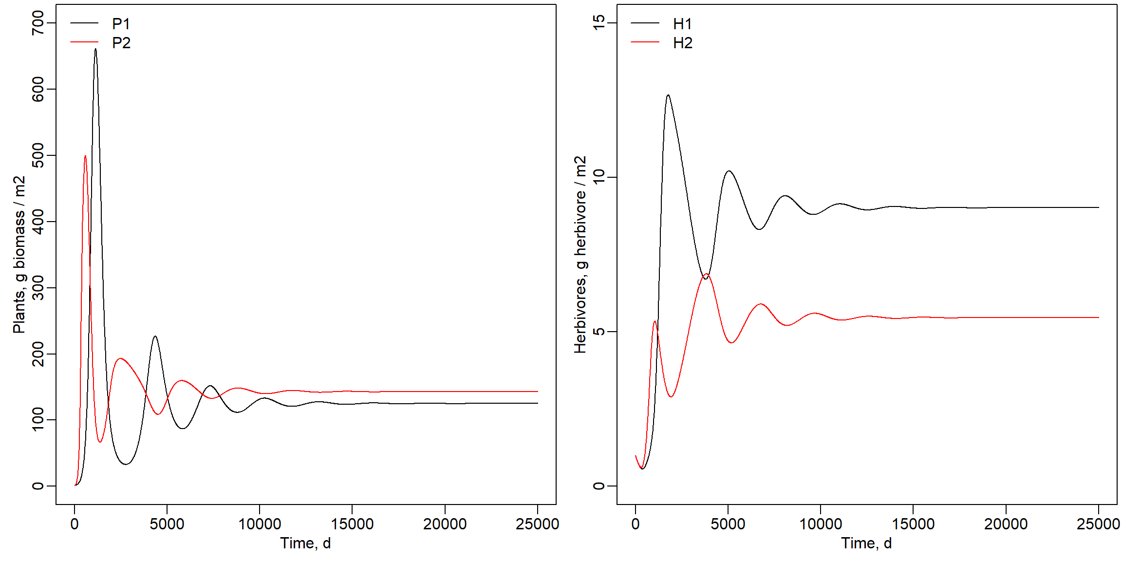
Indeed, the model did reach an equilibrium. We can also inspect the mass balance:
# compute mass balance in grams
MBForSpace_ode45 <- MassBalanceForSpace(states_ode45,
                                        ini = InitForSpace(),
                                        parms = ParmsForSpace(A11 = setA11))

# plot mass balance balance after resetting plotting canvas
par(mfrow = c(1,1))
plot(MBForSpace_ode45[,"time"], MBForSpace_ode45[,"BAL"], type = "l", col = "black",
     xlab = "Time, d", ylab = "Balance, g biomass/m2", ylim = c(-5e-10, 5e-10))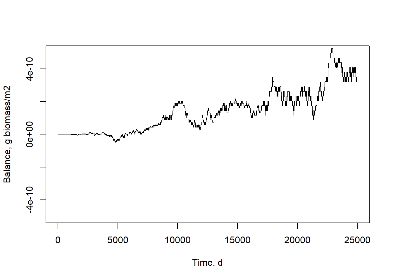
setA11 is defined that is used to set the parameter
A11 that defines the search rate of herbivore 1 for plant
species 1. Run the model after changing the value of this variable
setA11 to 0.004 and 0.008. How are the computed outcomes
affected by this parameter and how did this affect the equilibria in the
model? The values of the states and the equilibrium is affected by the value
for the parameter A11. The model did not yet reach an
equilibrium within 25000 days when A11 increased to 0.004
or 0.008 as shown below. The number of herbivores 1 and plant species 1
decreased, while plant species 2 ended up at about the same value. The
number of H2 strongly increased as shown below.
Parameter A11 set to value 0.004:
# Set AL1 here, to automatically change its value when used in the call to the ParmsForSpace function
setA11 <- 0.004 # 0.002 is the default

# Use deSolve to integrate derivatives numerically with Runge-Kutta and a variable time-step
states_ode45_004 <- ode(y = InitForSpace(),
                        time = seq(from = 0, to = 25000, by = 10),
                        func = RatesForSpace,
                        parms = ParmsForSpace(A11 = setA11),
                        method = "ode45")

# Define plotting settings
par(mfrow = c(1,2), # nr of rows and columns, filled by row. defaults to c(1,1)
    mar = c(3, 3, 0.25, 0.25), # margins mar = c(bottom, left, top, right), default is c(5, 4, 4, 2) + 0.1
    mgp = c(1.5, 0.5, 0)) # margin line mgp = c(axes text, label, line) in mex units, default is c(3, 1, 0)

# Plot the  states to compare vegetation and herbivores
plot(states_ode45_004[,"time"], states_ode45_004[,"P1"], type = "l", col = "black",
     xlim = c(0,25000), ylim = c(0,700), xlab = "Time, d", ylab = "Plants, g biomass / m2")
lines(states_ode45_004[,"time"], states_ode45_004[,"P2"], type = "l", col = "red")
legend("topleft", lty = 1, col = c("black","red"), legend = c("P1","P2"), bty = "n")

plot(states_ode45_004[,"time"], states_ode45_004[,"H1"], type = "l", col = "black",
     xlim = c(0,25000), ylim = c(0,15), xlab = "Time, d", ylab = "Herbivores, g herbivore / m2")
lines(states_ode45_004[,"time"], states_ode45_004[,"H2"],type = "l",col = "red")
legend("topleft", lty = 1, col = c("black","red"), legend = c("H1","H2"), bty = "n")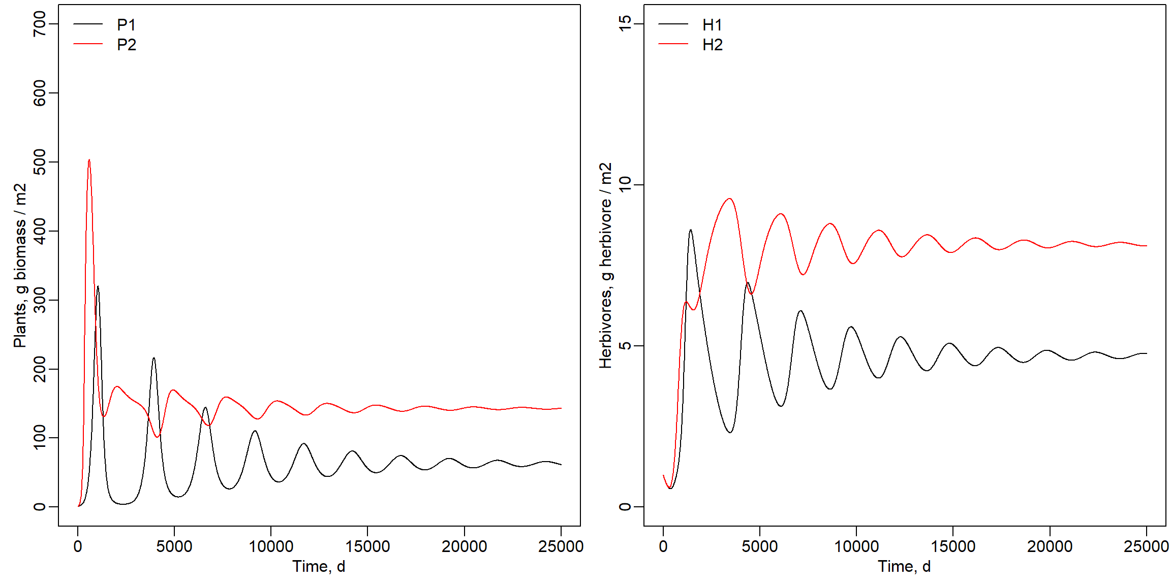
Parameter A11 set to value 0.008:
# Set AL1 here, to automatically change its value when used in the call to the ParmsForSpace function
setA11 <- 0.008 # 0.002 is the default

# Use deSolve to integrate derivatives numerically with Runge-Kutta and a variable time-step
states_ode45_008 <- ode(y = InitForSpace(),
                        time = seq(from = 0, to = 25000, by = 10),
                        func = RatesForSpace,
                        parms = ParmsForSpace(A11 = setA11),
                        method = "ode45")

# Define plotting settings
par(mfrow = c(1,2), # nr of rows and columns, filled by row. defaults to c(1,1)
    mar = c(3, 3, 0.25, 0.25), # margins mar = c(bottom, left, top, right), default is c(5, 4, 4, 2) + 0.1
    mgp = c(1.5, 0.5, 0)) # margin line mgp = c(axes text, label, line) in mex units, default is c(3, 1, 0)

# Plot the  states to compare vegetation and herbivores
plot(states_ode45_008[,"time"], states_ode45_008[,"P1"], type = "l", col = "black",
     xlim = c(0,25000), ylim = c(0,700), xlab = "Time, d", ylab = "Plants, g biomass / m2")
lines(states_ode45_008[,"time"], states_ode45_008[,"P2"], type = "l", col = "red")
legend("topleft", lty = 1, col = c("black","red"), legend = c("P1","P2"), bty = "n")

plot(states_ode45_008[,"time"], states_ode45_008[,"H1"], type = "l", col = "black",
     xlim = c(0,25000), ylim = c(0,15), xlab = "Time, d", ylab = "Herbivores, g herbivore / m2")
lines(states_ode45_008[,"time"], states_ode45_008[,"H2"],type = "l",col = "red")
legend("topleft", lty = 1, col = c("black","red"), legend = c("H1","H2"), bty = "n")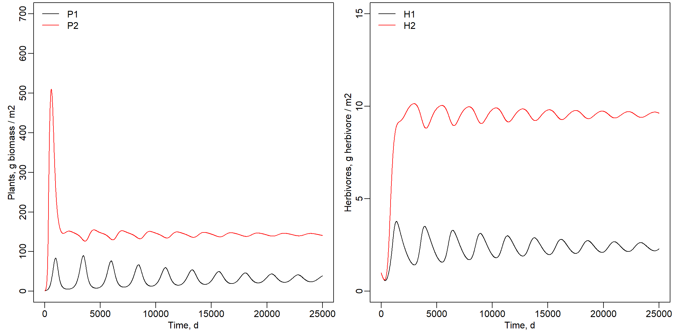
# Reset plotting settings (to their default values)
par(mfrow = c(1,1),
    mar = c(5, 4, 4, 2) + 0.1,
mgp = c(3, 1, 0)) Increasing the parameter
increased the preference for by
. Therefore more of was available for . is
only eaten by and this increase of
the A11 parameter increased the pressure on by
grazing. The reduced pressure on
from grazing was compensated by more
grazing. Note that herbivore 2 is
more effective in searching for this
when compared to as the parameter
value for is half the value of
parameter .
Exercise 9.2
In the previous exercise, we use the “ode45” solver: a 4th order Runge-Kutta solver with a variable timestep, so that during times of rapid system changes, the integration will automatically make smaller time-steps). In this exercise you are going to compare the outcomes of a model integrated with the “ode45” solver with outputs of Euler integration with different time-steps. We are looking for time-step convergence: solving a ODE model with Euler integration and with smaller time-steps should approximate true dynamics better (thus: with smaller time-steps, Euler integration should become closer to a solution with “ode45” integration). Time-step convergence is a way of checking whether the numerical solution of an ODE model is accurate and stable as you make the time-step smaller.
Evaluate how the differences between that outcomes are affected by a
smaller or larger time-step when using Euler integration. For this you
may want to change the time-steps between 100 and 1 days. Use the
lines function to add the state outcomes for and
and and to the plots as already created above. Set
the x-axis range to 0 - 2500 days. Use the same colors but now with
different line types (e.g. set lty = 1 for a solid line,
lty = 2 for a dashed line, etc; also value 3, 4 etc can be
used).
Comparison of ode45 and Euler with a time step of 1, 10 and 100 days. Indeed, with smaller time step during Euler integration, the model is converging with solutions ever closer to the “ode45” solution. This is expected, as we expect that errors are bigger if the rates are kept constant for longer time steps, while in reality they change continuously, even at infinitely small timesteps. Note that also the “ode45” solution will have some error when compared to a analytic solution, although this error will be very small.
# Set parameter A11 to default value
setA11 <- 0.002 # 0.002 is the default

# Solve with Euler and varyiing time steps
states_euler1 <- ode(y = InitForSpace(),
                    time = seq(from = 0, to = 2500, by = 1),
                    func = RatesForSpace,
                    parms = ParmsForSpace(A11 = setA11),
                    method = "euler")
states_euler10 <- ode(y = InitForSpace(),
                    time = seq(from = 0, to = 2500, by = 10),
                    func = RatesForSpace,
                    parms = ParmsForSpace(A11 = setA11),
                    method = "euler")
states_euler100 <- ode(y = InitForSpace(),
                    time = seq(from = 0, to = 2500, by = 100),
                    func = RatesForSpace,
                    parms = ParmsForSpace(A11 = setA11),
                    method = "euler")

# Define plotting settings
# Use the help function to understand what this function call using "par" does!
# Plot the states as function of time, with narrow plot margins.
par(mfrow = c(1,2), # nr of rows and columns, filled by row. defaults to c(1,1)
    mar = c(3, 3, 0.25, 0.25), # margins mar = c(bottom, left, top, right), default is c(5, 4, 4, 2) + 0.1
    mgp = c(1.5, 0.5, 0)) # margin line mgp = c(axes text, label, line) in mex units, default is c(3, 1, 0)

# Plot the  states to compare vegetation and herbivores
plot(states_ode45[,"time"], states_ode45[,"P1"], type = "l", col = "black",
     xlim = c(0,2500), ylim = c(0,800), xlab = "Time, d", ylab = "Plants, g biomass / m2")
lines(states_ode45[,"time"], states_ode45[,"P2"], type = "l", col = "red")
# Add euler solutions with different line types (but same colours)
# 1 time unit
lines(states_euler1[,"time"], states_euler1[,"P1"], type = "l", col = "black", lty = 2)
lines(states_euler1[,"time"], states_euler1[,"P2"], type = "l", col = "red", lty = 2)
# 10 time units
lines(states_euler10[,"time"], states_euler10[,"P1"], type = "l", col = "black", lty = 3)
lines(states_euler10[,"time"], states_euler10[,"P2"], type = "l", col = "red", lty = 3)
# 100 time unit
lines(states_euler100[,"time"], states_euler100[,"P1"], type = "l", col = "black", lty = 4)
lines(states_euler100[,"time"], states_euler100[,"P2"], type = "l", col = "red", lty = 4)
# Add legend (colour for state, linetype for method)
legend("topleft", title = "Solver", col = "grey",
       legend = c("ode45","Euler 1", "Euler 10", "Euler 100"), lty = 1:4, bty = "n")
legend("topright", title = "State", col = c("black","red"),
       legend = c("P1", "P2"), lty = 1, bty = "n")

# Plot the  states to compare vegetation and herbivores
plot(states_ode45[,"time"], states_ode45[,"H1"], type = "l", col = "black",
     xlim = c(0,2500), ylim = c(0,15), xlab = "Time, d", ylab = "Plants, g biomass / m2")
lines(states_ode45[,"time"], states_ode45[,"H2"], type = "l", col = "red")
# Add euler solutions with different line types (but same colours)
# 1 time unit
lines(states_euler1[,"time"], states_euler1[,"H1"], type = "l", col = "black", lty = 2)
lines(states_euler1[,"time"], states_euler1[,"H2"], type = "l", col = "red", lty = 2)
# 10 time units
lines(states_euler10[,"time"], states_euler10[,"H1"], type = "l", col = "black", lty = 3)
lines(states_euler10[,"time"], states_euler10[,"H2"], type = "l", col = "red", lty = 3)
# 100 time unit
lines(states_euler100[,"time"], states_euler100[,"H1"], type = "l", col = "black", lty = 4)
lines(states_euler100[,"time"], states_euler100[,"H2"], type = "l", col = "red", lty = 4)
# Add legend (colour for state, linetype for method)
legend("topleft", title = "Solver", col = "grey",
       legend = c("ode45","Euler 1", "Euler 10", "Euler 100"), lty = 1:4, bty = "n")
legend("topright", title = "State", col = c("black","red"),
       legend = c("H1", "H2"), lty = 1, bty = "n")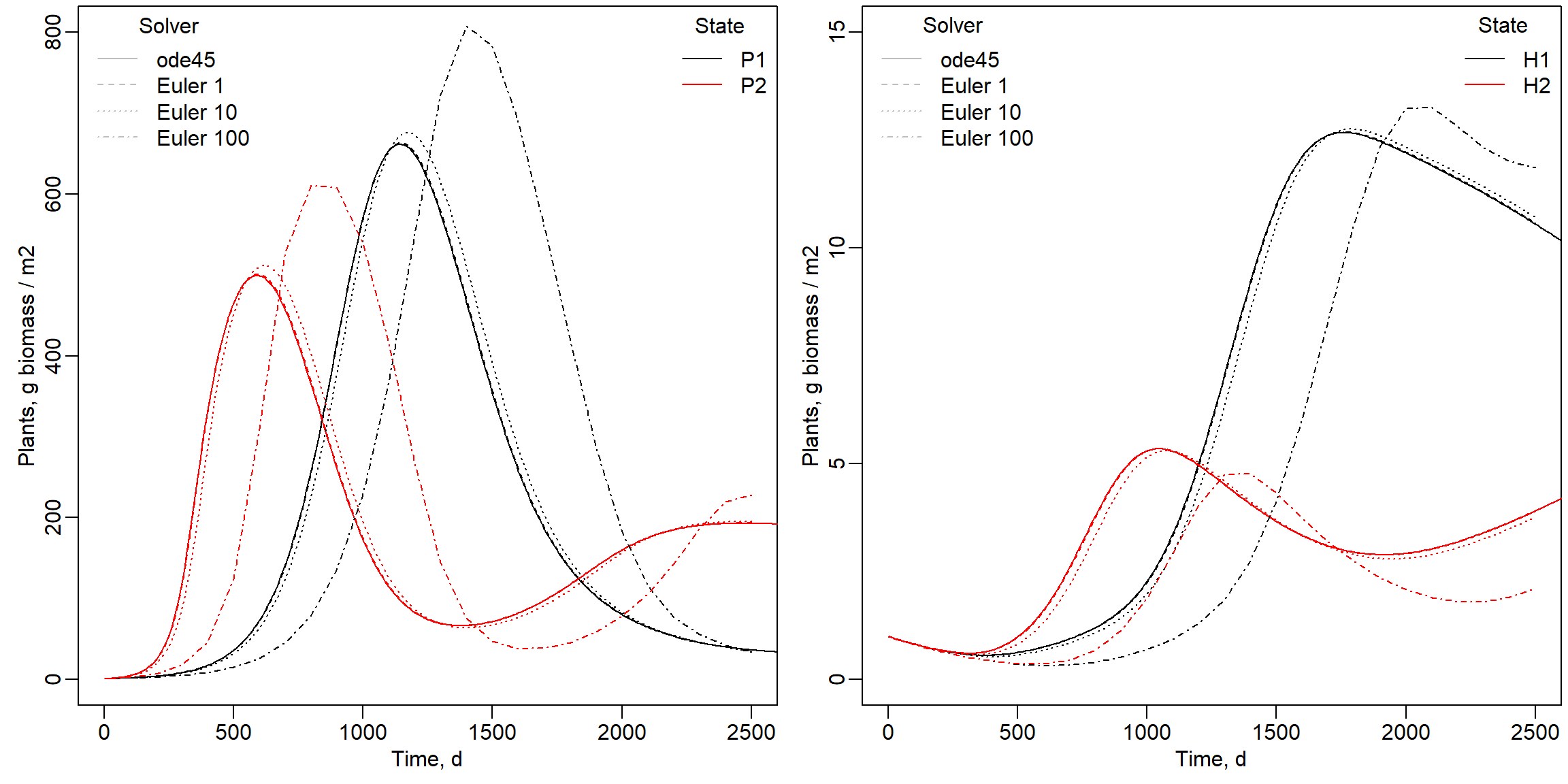
Exercise 9.3
Consider the following statements from a model that attempts to study the dynamics in the number of people with a Covid infection. The actual model that was developed includes different cohorts of people, and additional auxiliary variables, but that is ignored for this exercise.
The model tracks the following states: the unprotected persons () in the population, the infected () but not (yet) infectious persons, the infectious () persons and, sick (), hospitalised (), immune () and deceased () persons. All rates are expressed in persons per day:
Please work on paper to address the questions below!
When you set inputs to 0 the rate equations for , , , and are reflecting a situation with exponential decrease. For however this is not the case, here outflow depends on the number of persons, while for there is no outflow.
The TC is a system characteristic and does not depend on the inflow. With input set to 0, equilibrium values are 0 for , , , and . The inputs in the rate equations then also become 0 and fall away in these equations.
For : , as and .
This approach works as well for the other states.
For :
For :
For , without inflow the rate equation simplifies rate equation to:
Likewise for : .
For exponential equations, ART = TC and with equations from question 9.3b for IF, ART = 1/(1/300) = 300 days.
For exponential equations, ART = TC. With an ART of 3, TC = 3 and rinfdr = 1/3 d-1
For in equilibrium the state also needs to be in equilibrium:
For :
A more challenging question:
The number of people that will be infected by 1 person can be determined by looking at a component of the rate equation for . Note that there was only one person infectious that remains infectious for a short period of time. The average residence time for , so a person is infectious for on average only 3 days (see 9.3d). Note that the parameter had a value of 1/3. With one infected person equals 1 and we can use this rate equation:
The total number of people that will be infected by this person, the R number, can be found by integrating this rate equation from 0 to 3 days:
It can be easily understood that with e.g. 60 person to person encounters per day and a relative infection rate of 0.01 each day 0.6 other persons are infected resulting in an R value of 1.8. A new virus strain with an of 0.02 will result in an R value of 60 * 0.02 * 3 = 3.6.
Solutions as R script
Download here the code as shown on this page in a separate .r file.