Wageningen University & Research | FEM-31806 | Models for Ecological Systems | FEM | PPS | WEC

Aims

Implement the model

Implement the mini-Nucom model in R. Use the equations as defined in the mini-model documents. Set up a basic structure to implement the model in R, using the provided R templates. Recall that this means defining (at least) 3 functions that will provide the main input to the deSolve ode function that will be used to numerically solve the model:
- One function that defines the parameter values of the model: call the function “ParmsNUCOM”, this function will provide input to the ode input argument parms;
- One function that defines the initial values of the state variables (call the function “InitNUCOM”, this function will provide input to the ode input argument y;
- One function that defines the auxiliary variables and rates equations for all states variables (call the function “RatesNUCOM”, this function will be the input to the ode input argument func.

Perform technical tests

Run the model for default parameters and initial state values. Check for any programming errors, including possible zero divisions or discontinuities. Ensure to run it for a sufficiently long period of time, e.g. 150 years, to check if the model reached an equilibrium or resulted in odd behaviour. Run the model using an adaptive stepsize Runge-Kutta integration method: method “ode45”.
Once there are no programming errors, plot the state variables against time: this helps for showing possible left errors. Importantly: does the simulation results reflect the intentions of the model developers?
Vary values of one key parameter. Before doing so, consider the possible effect of this on the state variable – time plots. Make the plots for the default model, but adapted for that single parameter value, and check whether the results follow your expectation. You can repeat this for another key parameter. If the model performs according your expectation, this gives further trust in the model.
Investigate the equilibria in your ecological system by evaluating the state variable – time plots. Does the system come in equilibrium? If not, try longer time periods for the simulation. Does the system ultimately come in equilibrium? If not, why not?
The rate of change of the state variable(s) should not change any longer in equilibrium. Plot therefore the state rates against time. Do these plots correspond with the state – time plots, and show the same results for equilibria?
Do you expect equilibria to differ (reach alternative stable states) when starting with different initial values? If so, vary initial values and check for existence of alternative equilibria.
Check if the computed values for state variables in equilibrium indeed result in rates with a value of 0, as additional check for the implemented formulas. Do this by filling in the computed results in the mathematical equations.
Analyse model behaviour for extreme values of some parameters. Does the model still run correctly, or will there be errors? Is the output what you expect?

Answers

Download here the code as shown on this page in a separate .r file.

Implement the model

See the Templates providing a structure to implement a model in R.

Parameters

The function returning a named vector with parameter values:

ParmsNUCOM <- function(
  ### Inputs from outside into the system

  # Nitrogen from atmospheric deposition
  NDEPCO = 2.0,  # gN / (m2 * year)
  # Imported carbon from seeds from outside the considered field
  SEEDC1 = 10.0, # gC / (m2 year)
  SEEDC2 = 10.0, # gC / (m2 year)

  # Imported nitrogen from seeds from outside the considered field
  SEEDN1 = 0.2, # gN / (m2 year) 
  SEEDN2 = 0.2, # gN / (m2 year)

  ### System parameter values
  
  # Nitrogen concentration in species 1 and 2
  NCONC1 = 0.02, # gN / gC
  NCONC2 = 0.02, # gN / gC

  # Maximum growth rate of species 1 and 2
  GMAX1 = 300.0, # gC / (m2 year)
  GMAX2 = 900.0, # gC / (m2 year)
  
  # Relative mortality rates of species 1 and 2
  MORT1 = 0.6, # (g/year) / g or 1/year
  MORT2 = 0.9, # (g/year) / g or 1/year

  # Relative decay rates of species 1 and 2
  DECAY1 = 0.1, # (g/year) / g or 1/year
  DECAY2 = 0.3, # (g/year) / g or 1/year
  
  # Carbon en nitrogen concentrations of the micro-organisms
  CCONMO = 0.5, # gC / g biomass
  NCONMO = 0.05, # gN / g biomass
  
  # Assimilation efficiency of the micro-organisms
  EFFMO = 0.2 # gCbuilt in into Biomass / gC liberated from soil organic matter
  ) {
  # Gather parameters in a named vector
  y <- c(NDEPCO = NDEPCO,
         SEEDC1 = SEEDC1, SEEDC2 = SEEDC2,
         SEEDN1 = SEEDN1, SEEDN2 = SEEDN2,
         NCONC1 = NCONC1, NCONC2 = NCONC2,
         GMAX1 = GMAX1, GMAX2 = GMAX2, 
         MORT1 = MORT1, MORT2 = MORT2, 
         DECAY1 = DECAY1, DECAY2 = DECAY2,
         CCONMO = CCONMO,
         NCONMO = NCONMO,
         EFFMO = EFFMO)
  
  # Return
  return(y)
}

Initial conditions

The function returning a named vector with initial values of the 8 state variables:

Biomass Carbon of two vegetation species (BC1, BC2);
Biomass Nitrogen of two vegetation species (BN1, BN2);
Soil Carbon coming from the two plant species (SC1, SC2);
Soil Nitrogen coming from the two plant species (SN1, SN2):

InitNUCOM <- function(
  # For the vegetation
  BC1 = 25.0,  # gC in Veg.1 / m2
  BC2 = 25.0,  # gC in Veg.2 / m2
  BN1 = 0.5,   # gN in Veg.1 / m2 
  BN2 = 0.5,   # gN in Veg.2 / m2
  
  # For the soil
  SC1 = 25.0, # gC from Veg.1 / m2 
  SC2 = 25.0, # gC from Veg.2 / m2
  SN1 = 0.5,  # gN from Veg.1 / m2
  SN2 = 0.5   # gN from Veg.2 / m2
){
  # Gather initial conditions in a named vector; given names are names for the state variables in the model
  y <- c(BC1 = BC1, BC2 = BC2,
         BN1 = BN1, BN2 = BN2,
         SC1 = SC1, SC2 = SC2,
         SN1 = SN1, SN2 = SN2)
  
  # Return
  return(y)
}

Differential equations

The function computing the rates of change of the state variables with respect to time:

RatesNUCOM <- function(t, y, parms) {
  # use the with() function to be able to access the parameters and states easily
  # remember that the with() function is with(data, expr), where
  # - 'data' is ideally a list with named elements
  #   thus: 'y' and 'parms' are combined using function c and converted using function as.list
  # - 'expr' is an expression (i.e. code) that is evaluated
  #   this can span multiple lines of code when embraced with curly brackets {}
  with(
    as.list(c(y, parms)),{
      
      ### Optional: forcing functions: get value of the driving variables at time t (if any)
      
      ### Optional: auxiliary equations
      
      # Litter production of both species in terms of Carbon and Nitrogen
      LITPC1 <- BC1 * MORT1
      LITPC2 <- BC2 * MORT2
      LITPN1 <- BN1 * MORT1
      LITPN2 <- BN2 * MORT2
      
      # Decomposition of soil organic matter in terms of carbon and nitrogen
      # DECOM is the net carbon production, lost as CO2-C from the system
      DECOM1 <- SC1 * DECAY1 * (1.0 - EFFMO)
      DECOM2 <- SC2 * DECAY2 * (1.0 - EFFMO)
  
      # Definition of details of overall input-output rate equations
      # Mineralisation of Nitrogen
      MINER1 <- DECAY1 * SC1*( (SN1/SC1) - (NCONMO/CCONMO)*EFFMO )
      MINER2 <- DECAY2 * SC2*( (SN2/SC2) - (NCONMO/CCONMO)*EFFMO )
      MINTOT <- MINER1 + MINER2
  
      # Nitrogen supply to (N-deposition) the system
      NDEP <- NDEPCO
      NAVAIL <- NDEP + MINER1 + MINER2
      
      # Growth rates of both species
      NLIMG1 <- ( BC1/(BC1 + BC2) ) * NAVAIL/NCONC1
      LLIMG1 <- ( BC1/(BC1 + BC2) ) * GMAX1
      ACTGC1 <- pmin(NLIMG1 , LLIMG1)
  
      NLIMG2 <- ( BC2/(BC1 + BC2) ) * NAVAIL/NCONC2
      LLIMG2 <- ( BC2/(BC1 + BC2) ) * GMAX2
      ACTGC2 <- pmin(NLIMG2 , LLIMG2)
      
      # Therefore, CO2 evolution is calculated per species and in total as:
      CO21DT <- DECOM1
      CO22DT <- DECOM2
      # TOTCO2 = CO21 + CO22
  
      # Nitrogen uptake rates of both species
      NUPT1 <- ACTGC1 * NCONC1
      NUPT2 <- ACTGC2 * NCONC2
    
      # Nitrogen loss (Leaching) from the system
      LEACH <- NAVAIL - NUPT1 - NUPT2

      ### Rate equations
      DBC1DT <- ACTGC1 - LITPC1 + SEEDC1
      DBC2DT <- ACTGC2 - LITPC2 + SEEDC2
      DBN1DT <- NUPT1 - LITPN1 + SEEDN1
      DBN2DT <- NUPT2 - LITPN2 + SEEDN2
      DSC1DT <- LITPC1 - DECOM1
      DSC2DT <- LITPC2 - DECOM2
      DSN1DT <- LITPN1 - MINER1
      DSN2DT <- LITPN2 - MINER2

      ### Gather all rates of change in a vector
      # - the rates should be in the same order as the states (as specified in 'y')
      # - it can be a named vector, but does not need to be
      RATES <- c(DBC1DT = DBC1DT,
                 DBC2DT = DBC2DT,
                 DBN1DT = DBN1DT,
                 DBN2DT = DBN2DT,
                 DSC1DT = DSC1DT,
                 DSC2DT = DSC2DT,
                 DSN1DT = DSN1DT,
                 DSN2DT = DSN2DT)
      
      ### Optional: get in/out flow used to compute mass balances (or set MB <- NULL)
      # not included here (thus here use MB <- NULL), see template 3
      MB <- NULL
      
      ### Optional: gather auxiliary variables that should be returned (or set AUX <- NULL)
      # - this should be a named vector or list!
      AUX <- NULL
      
      # Return result as a list
      # - the first element is a vector with the rates of change (in the same order as 'y')
      # - all other elements are (optional) extra output, which should be named
      outList <- list(c(RATES, # the rates of change of the state variables (same order as 'y'!)
                        MB),   # the rates of change of the mass balance terms (or NULL)
                      AUX) # optional additional output per time step
      return(outList)
    })
}

With these 3 functions now defined, the NUCOM mini-model has been implemented in R code, and the model can now numerically be solved using the ode function from the deSolve package.

Performing technical tests

Use deSolve to integrate the model numerically using Euler integration, here for 150 years in timesteps of 1.

states <- ode(y = InitNUCOM(),
              times = seq(from=0, to=150, by=1),
              parms = ParmsNUCOM(),
              func = RatesNUCOM,
              method = "euler")

Model checks

We split up the testing of the model implementation in two steps: by checking whether the model runs technically and whether the computed results are reasonable.

First, if a model implementation runs technically without errors or important warning messages, it means e.g. that there are no zero divisions and no unexpected discontinuities. We can assess this by plotting state variables versus time or versus each other. If this appears to be correct, we can assess whether the model implementation computes results that are reasonable. First, we can plot the computed results using:

plot(states)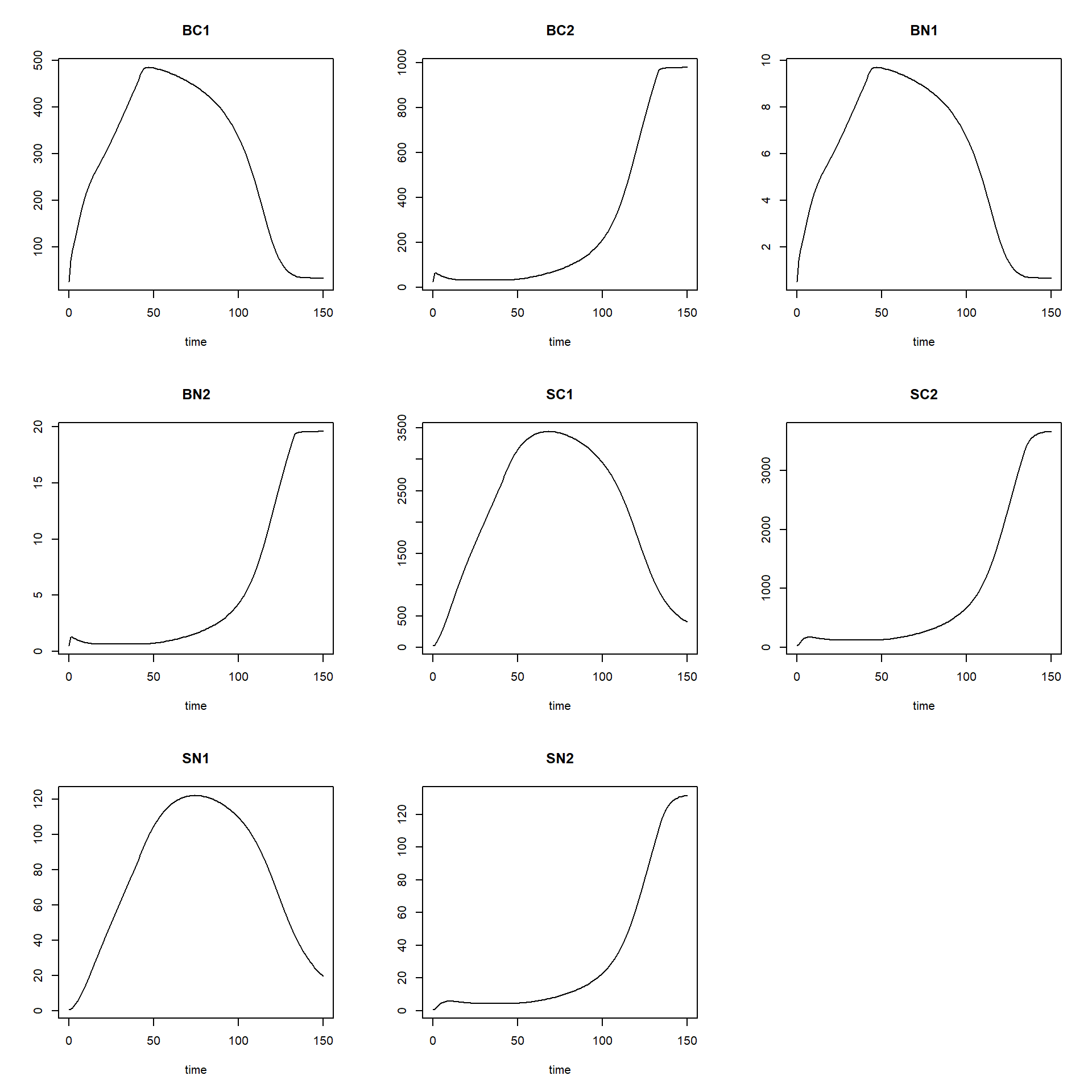

Second, we can check whether the results are reasonable by checking the units of the model implementation, similarly as for the model equations. Of course, if you did everything correctly, the units will be the same, but it is still needed and often programming errors are discovered. The reasonableness of results can also be checked if we know (or expect) that the model (and thus the model application) ought to reach an equilibrium. In that case the (net) rates will become zero. We can discover this by running the model for a long time period with small steps.

Some models will reach an equilibrium state after a period time. Often you have an expectation, if an equilibrium can be expected to occur.

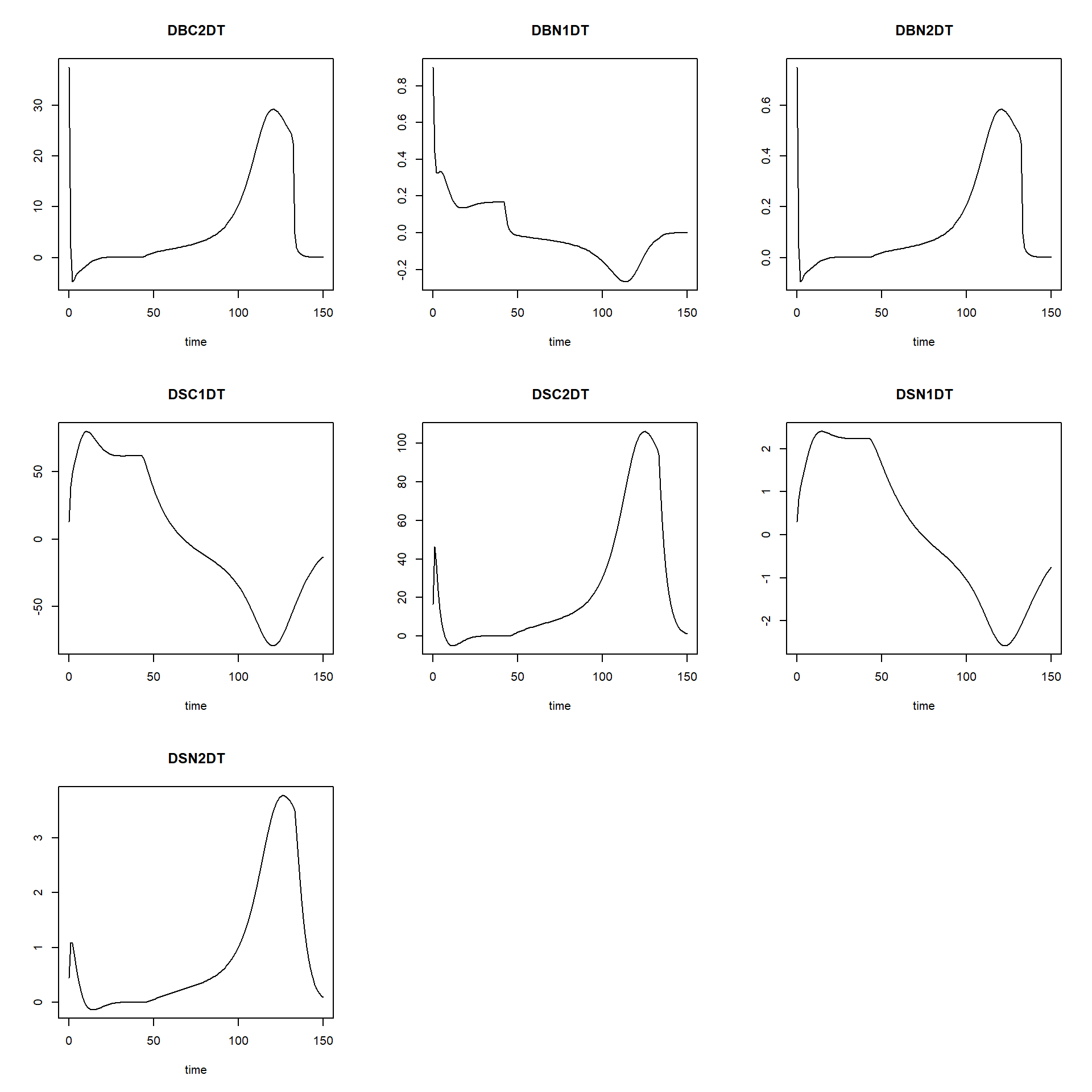
If we want to look at how the rates of change vary over time, and thus not only the values of the state variables, we can do this easily by changing AUX <- NULL into AUX <- RATES in the function defined above that computes the rates of change of the state variables. Then, simply running plot(states) will not only plot the state variables as function of time, but also their rates as function of time.

### SAME as earlier, but with AUX <- RATES
RatesNUCOM <- function(t, y, parms) {
  # use the with() function to be able to access the parameters and states easily
  # remember that the with() function is with(data, expr), where
  # - 'data' is ideally a list with named elements
  #   thus: 'y' and 'parms' are combined using function c and converted using function as.list
  # - 'expr' is an expression (i.e. code) that is evaluated
  #   this can span multiple lines of code when embraced with curly brackets {}
  with(
    as.list(c(y, parms)),{
      
      ### Optional: forcing functions: get value of the driving variables at time t (if any)
      
      ### Optional: auxiliary equations
      
      # Litter production of both species in terms of Carbon and Nitrogen
      LITPC1 <- BC1 * MORT1
      LITPC2 <- BC2 * MORT2
      LITPN1 <- BN1 * MORT1
      LITPN2 <- BN2 * MORT2
      
      # Decomposition of soil organic matter in terms of carbon and nitrogen
      # DECOM is the net carbon production, lost as CO2-C from the system
      DECOM1 <- SC1 * DECAY1 * (1.0 - EFFMO)
      DECOM2 <- SC2 * DECAY2 * (1.0 - EFFMO)
  
      # Definition of details of overall input-output rate equations
      # Mineralisation of Nitrogen
      MINER1 <- DECAY1 * SC1*( (SN1/SC1) - (NCONMO/CCONMO)*EFFMO )
      MINER2 <- DECAY2 * SC2*( (SN2/SC2) - (NCONMO/CCONMO)*EFFMO )
      MINTOT <- MINER1 + MINER2
  
      # Nitrogen supply to (N-deposition) the system
      NDEP <- NDEPCO
      NAVAIL <- NDEP + MINER1 + MINER2
      
      # Growth rates of both species
      NLIMG1 <- ( BC1/(BC1 + BC2) ) * NAVAIL/NCONC1
      LLIMG1 <- ( BC1/(BC1 + BC2) ) * GMAX1
      ACTGC1 <- pmin(NLIMG1 , LLIMG1)
  
      NLIMG2 <- ( BC2/(BC1 + BC2) ) * NAVAIL/NCONC2
      LLIMG2 <- ( BC2/(BC1 + BC2) ) * GMAX2
      ACTGC2 <- pmin(NLIMG2 , LLIMG2)
      
      # Therefore, CO2 evolution is calculated per species and in total as:
      CO21DT <- DECOM1
      CO22DT <- DECOM2
      # TOTCO2 = CO21 + CO22
  
      # Nitrogen uptake rates of both species
      NUPT1 <- ACTGC1 * NCONC1
      NUPT2 <- ACTGC2 * NCONC2
    
      # Nitrogen loss (Leaching) from the system
      LEACH <- NAVAIL - NUPT1 - NUPT2

      ### Rate equations
      DBC1DT <- ACTGC1 - LITPC1 + SEEDC1
      DBC2DT <- ACTGC2 - LITPC2 + SEEDC2
      DBN1DT <- NUPT1 - LITPN1 + SEEDN1
      DBN2DT <- NUPT2 - LITPN2 + SEEDN2
      DSC1DT <- LITPC1 - DECOM1
      DSC2DT <- LITPC2 - DECOM2
      DSN1DT <- LITPN1 - MINER1
      DSN2DT <- LITPN2 - MINER2

      ### Gather all rates of change in a vector
      # - the rates should be in the same order as the states (as specified in 'y')
      # - it can be a named vector, but does not need to be
      RATES <- c(DBC1DT = DBC1DT,
                 DBC2DT = DBC2DT,
                 DBN1DT = DBN1DT,
                 DBN2DT = DBN2DT,
                 DSC1DT = DSC1DT,
                 DSC2DT = DSC2DT,
                 DSN1DT = DSN1DT,
                 DSN2DT = DSN2DT)
      
      ### Optional: get in/out flow used to compute mass balances (or set MB <- NULL)
      # not included here (thus here use MB <- NULL), see template 3
      MB <- NULL
      
      ### Optional: gather auxiliary variables that should be returned (or set AUX <- NULL)
      # - this should be a named vector or list!
      AUX <- RATES
      
      # Return result as a list
      # - the first element is a vector with the rates of change (in the same order as 'y')
      # - all other elements are (optional) extra output, which should be named
      outList <- list(c(RATES, # the rates of change of the state variables (same order as 'y'!)
                        MB),   # the rates of change of the mass balance terms (or NULL)
                      AUX) # optional additional output per time step
      return(outList)
    })
}

# solve the model
states <- ode(y = InitNUCOM(),
              times = seq(from = 0, to = 150, by = 1),
              parms = ParmsNUCOM(),
              func = RatesNUCOM,
              method = "euler")

# explore
head(states)

##      time       BC1      BC2      BN1      BN2      SC1      SC2      SN1      SN2   DBC1DT    DBC2DT    DBN1DT      DBN2DT   DSC1DT    DSC2DT   DSN1DT
## [1,]    0  25.00000 25.00000 0.500000 0.500000  25.0000  25.0000 0.500000 0.500000 45.00000 37.500000 0.9000000  0.75000000 13.00000 16.500000 0.300000
## [2,]    1  70.00000 62.50000 1.400000 1.250000  38.0000  41.5000 0.800000 0.950000 21.88679  1.863208 0.4377358  0.03726415 38.96000 46.290000 0.836000
## [3,]    2  91.88679 64.36321 1.837736 1.287264  76.9600  87.7900 1.636000 2.039000 16.45824 -4.785207 0.3291649 -0.09570414 48.97528 36.857287 1.092962
## [4,]    3 108.34504 59.57800 2.166901 1.191560 125.9353 124.6473 2.728962 3.112578 16.18878 -4.470243 0.3237756 -0.08940486 54.93220 23.704852 1.279115
## [5,]    4 124.53382 55.10776 2.490676 1.102155 180.8675 148.3521 4.008076 3.999092 16.68932 -3.572219 0.3337864 -0.07144439 60.25089 13.992468 1.455333
## [6,]    5 141.22314 51.53554 2.824463 1.030711 241.1184 162.3446 5.463409 4.681417 16.64351 -3.036294 0.3328702 -0.06072588 65.44441  7.419279 1.630573
##         DSN2DT
## [1,] 0.4500000
## [2,] 1.0890000
## [3,] 1.0735777
## [4,] 0.8865144
## [5,] 0.6823248
## [6,] 0.4972822

plot(states)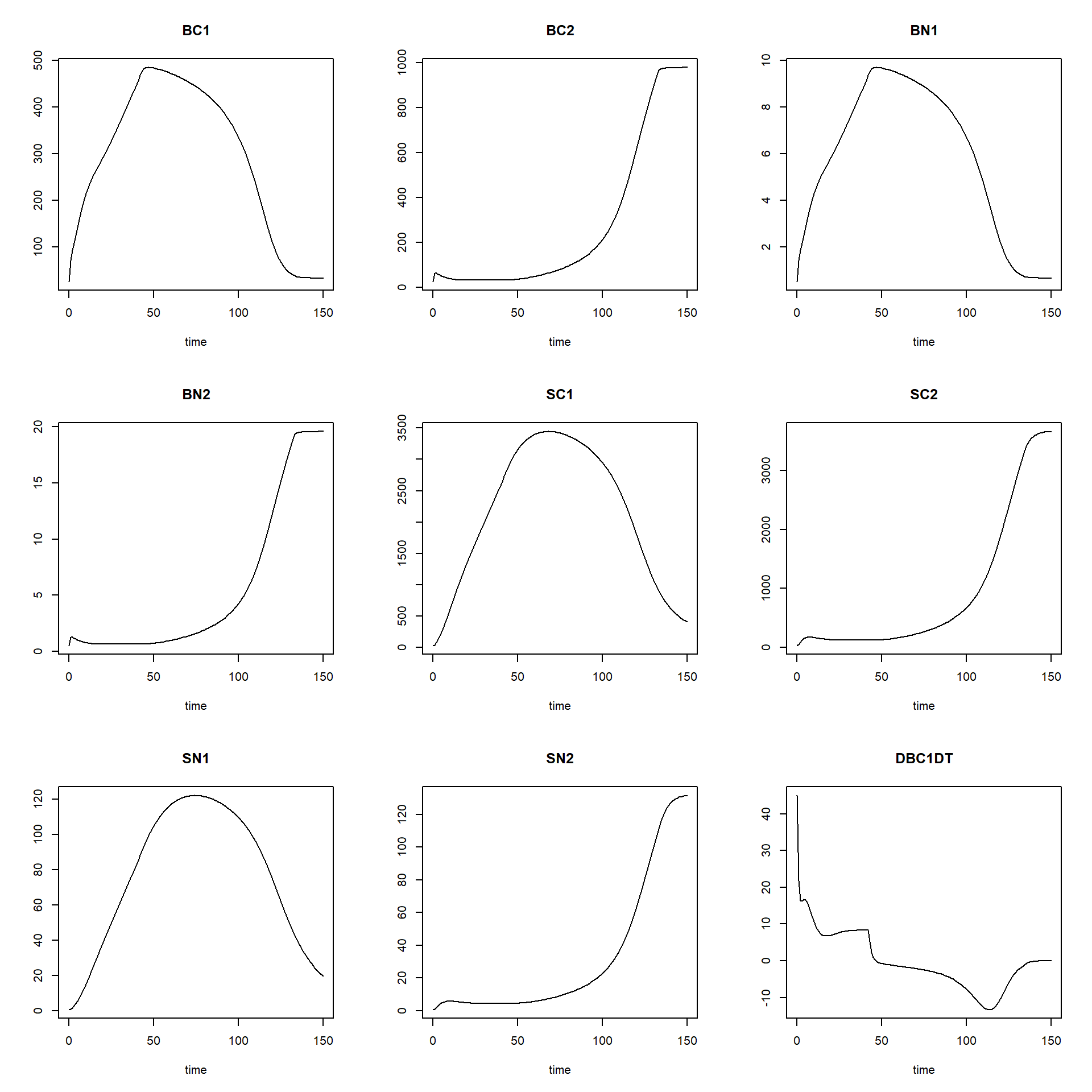

Moreover, we can easily change parameter values or initial state values from their defaults, by including input values to the function calls to functions “ParmsNUCOM” (input to the argument parms in the ode function call), as well as function “InitNUCOM” (input to the argument y in the ode function call).

NUCOM - Day 2

Aims

Implement the model

Perform technical tests

Answers

Implement the model

Parameters

Initial conditions

Differential equations

Performing technical tests