Wageningen University & Research | FEM-31806 | Models for Ecological Systems | FEM | PPS | WEC
Chapter 8 - Calibration and evaluation
Knowledge questions
A model that is too simple often does not perform well because it cannot capture the true structure of the system: it systematically misses important structure.
A more complex model sounds like it should perform better: more parameters, more flexibility, more ability to capture patterns. But in practice, complexity can easily become a liability, because a more complex model also will involve more parameters, which likely will have uncertainty of themselves, and which may thus need to be estimated using (perhaps limited) data. Everything else being equal, properly calibrating a more complex model is more challenging than calibrating a simple model with fewer parameters. A model can even be too complex, in that multiple components/parameters capture the same pattern, leading to identifiability (and thus calibration) issues. According to the KISS principle, a model should be kept as simple as possible - avoiding unnecessary complexity - because simpler models are easier to understand, calibrate, and often generalize better.
Using the same dataset for both calibrating and evaluating a model is not a wise idea. It gives an overly optimistic impression of performance because the model is being tested on data it has already seen (during calibration). A better approach is to evaluate the model on data that was not used during calibration.
Exercise 8.1
In this practical, we continue with the model, data and scripts used during yesterday’s practical (exercise 7.1). Besides the information given in exercise 7.1, Template 6 may come in handy today! A short recap on the previous exercise: we will thus use the logistic growth function again; where the rate of change of the population is given by:
where the parameter is the intrinsic (relative) growth rate and is the carrying capacity, which is not constant over time, but relates in a linear fashion to a driving variable (e.g. the amount of resources available):
Assume that all parameter values, state variables and driving variables have values > 0. As in exercise 7.1, assume that our initial values are as follows , , and . As before, measurements (at discreate points in time) on and are as follows:
surveyData <- data.frame(t = 0:50,
                         R = c(84,82,53,67,74,123,150,136,92,105,120,136,144,117,
                               120,136,125,93,108,123,113,149,112,112,51,64,109,
                               112,98,115,90,102,65,50,63,66,125,150,121,120,125,
                               120,121,139,113,96,115,82,97,101,85),
                         N = c(5,7,8,10,13,14,20,23,27,30,35,44,46,50,49,56,54,55,
                               57,56,58,62,58,54,47,47,42,47,48,48,51,54,51,43,36,
36,37,39,51,50,55,48,53,61,62,61,52,55,53,47,48)) # Load dataset
surveyData <- data.frame(t = 0:50,
R = c(84,82,53,67,74,123,150,136,92,105,120,136,144,117,
120,136,125,93,108,123,113,149,112,112,51,64,109,
112,98,115,90,102,65,50,63,66,125,150,121,120,125,
120,121,139,113,96,115,82,97,101,85),
N = c(5,7,8,10,13,14,20,23,27,30,35,44,46,50,49,56,54,55,
57,56,58,62,58,54,47,47,42,47,48,48,51,54,51,43,36,
36,37,39,51,50,55,48,53,61,62,61,52,55,53,47,48))
# Define a function that returns a named vector with initial state values
InitLogistic <- function(N = 5) {
# Gather function arguments in a named vector
y <- c(N = N)
# Return the named vector
return(y)
}
# Define a function that returns a named vector with parameter values
ParmsLogistic <- function(r = 0.25, # intrinsic population growth rate
k0 = 20, # intercept of the carrying capacity
k1 = 0.2 # slope of the carrying capacity with R
) {
# Gather function arguments in a named vector
y <- c(r = r,
k0 = k0,
k1 = k1)
# Return the named vector
return(y)
}
# Define the forcing function using the data as loaded above
R_linear <- approxfun(x = surveyData$t, y = surveyData$R, method = "linear", rule = 2)
# Define a function for the rates of change of the state variables with respect to time
RatesLogistic <- function(t, y, parms) {
with(
as.list(c(y, parms)),{
# Optional: forcing functions: get value of the driving variables at time t (if any)
R <- R_linear(t)
# Optional: auxiliary equations
K <- k0 + k1*R
# Rate equations
dNdt <- r * N * (1 - N / K)
# Gather all rates of change in a vector
RATES <- c(dNdt = dNdt)
# Optional: get in/out flow used to compute mass balances (or set MB <- NULL)
MB <- NULL
# Optional: gather auxiliary variables that should be returned (or set AUX <- NULL)
AUX <- c(R = R,
K = K)
# Return result as a list
outList <- list(c(RATES, # the rates of change of the state variables (same order as 'y'!)
MB), # the rates of change of the mass balance terms (or NULL)
AUX) # optional additional output per time step
return(outList)
}
)
}
# Numerically solve the model using the ode() function
states <- ode(y = InitLogistic(),
times = surveyData$t,
func = RatesLogistic,
parms = ParmsLogistic(),
method = "ode45")
# Plot the results
plot(states[,"time"], states[,"N"], type = "l", xlab = "time", ylab = "N", ylim = c(0, 75))
points(surveyData$t, surveyData$N)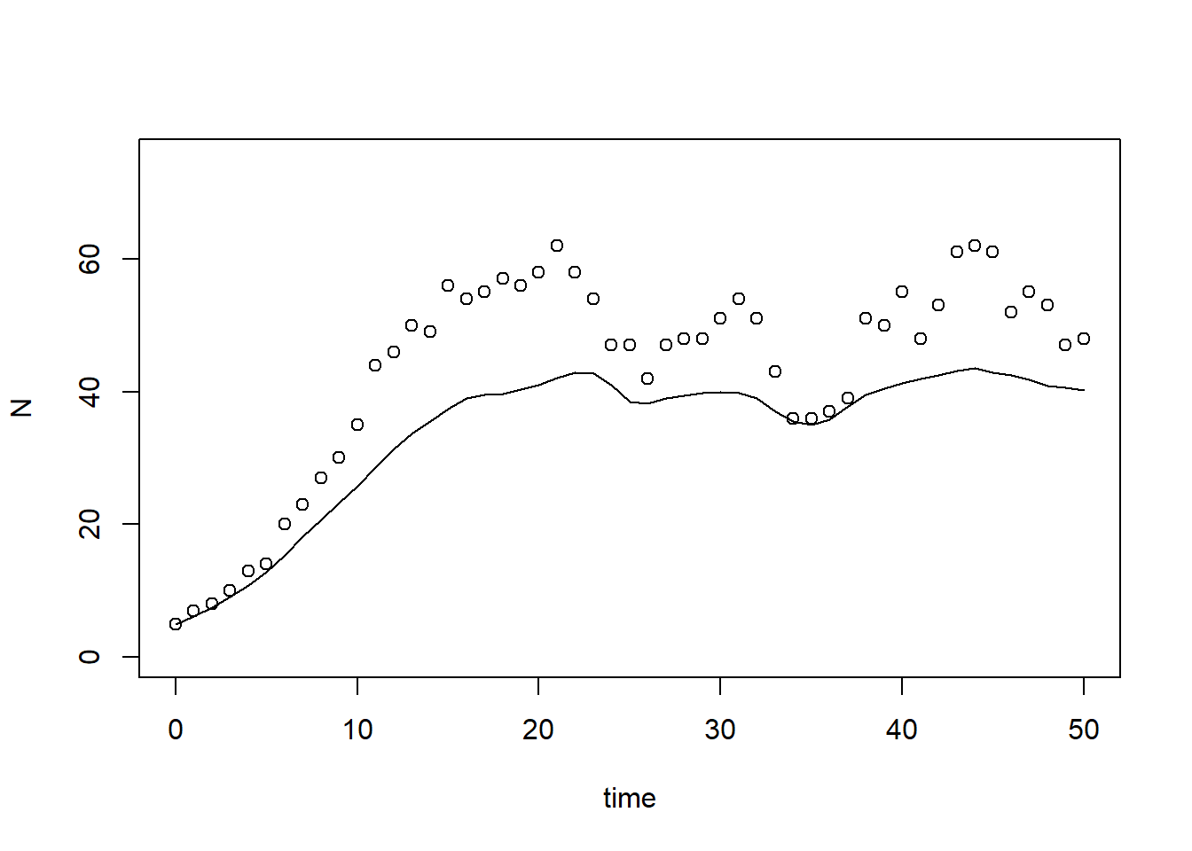
predictionError) that computes
the prediction error: the model’s prediction (given parameter values and
initial condition) minus the observed data (observations at specified
points in time). The function should thus first solve the model
numerically (for this you will need at least 4 inputs: the parameter
values, the initial state values, the times at which you want the
output, and the function returning the rates of change of the state
variables). Then, you need to subtract the observed value of the state
from the predicted value of state
at all points in time for which you
have measurements. Therefore: request model output for the times listed
in surveyData. # Define a function that computes prediction errors
predictionError <- function(p, # the parameters
y0, # the initial conditions
fn, # the function with rate equation(s)
name, # the name of the state parameter
obs_values, # the measured state values
obs_times, # the time-points of the measured state values
out_time = seq(from = 0, # times for the numerical integration
to = max(obs_times), # default: 0 - max(obs_times)
by = 1) # in steps of 1
) {
# Get out_time vector to retrieve predictions for (combining 'obs_times' and 'out_time')
out_time <- unique(sort(c(obs_times, out_time)))
# Solve the model to get the prediction
pred <- ode(y = y0,
times = out_time,
func = fn,
parms = p,
method = "ode45")
# NOTE: in case of a 'stiff' problem, method "ode45" might result in an error that the max nr of
# iterations is reached. Using method "rk4" (fixed timestep 4th order Runge-Kutta) might solve this.
# Get predictions for our specific state, at times t
pred_t <- subset(pred, time %in% obs_times, select = name)
# Compute errors, err: prediction - obs
err <- pred_t - obs_values
# Return
return(err)
}# Compute prediction error
err <- predictionError(p = ParmsLogistic(),
y0 = InitLogistic(),
fn = RatesLogistic,
name = "N",
obs_values = surveyData$N,
obs_times = surveyData$t)
# Plot prediction error over time
plot(surveyData$t, err, xlab = "time", ylab = "prediction error")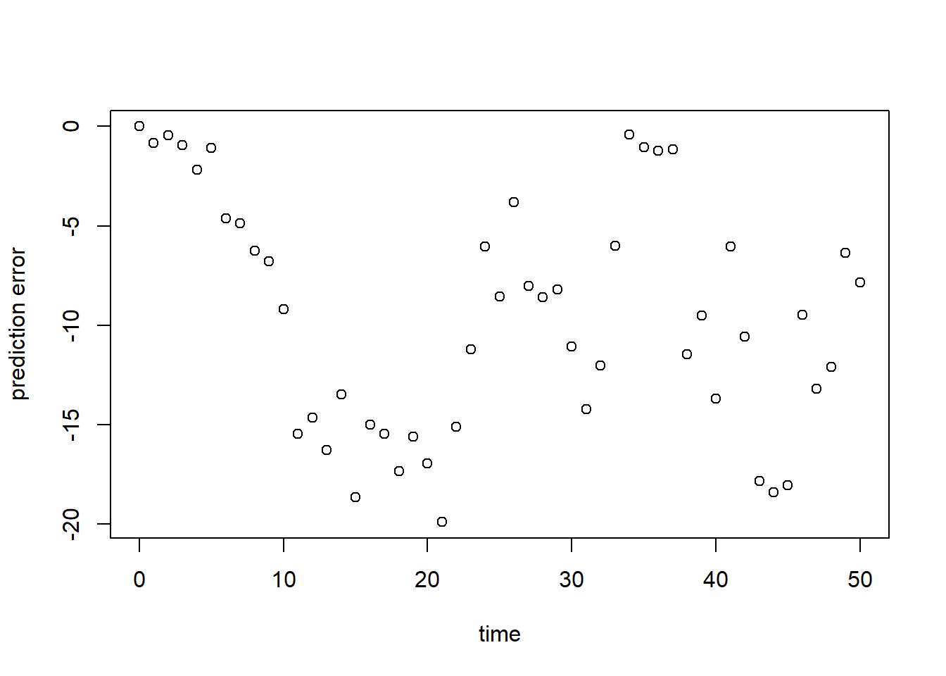
As can be seen here, but also already in the plot in exercise 8.1a, the model at its default values does have a large error, and systematically underestimates the population’s size.
sqrt(mean(err^2))## [1] 11.21278Similar to the above, we see a poor model fit (RMSE is ca. 11.21). Relative to the average population size (say 50), this error is large!
Define a function called predRMSE that computes the RMSE
when you provide it with at least the following information:
- Parameter values, which are unconstrained in their values (i.e. they can have any value in the range to );
- Initial state values;
- The function calculating the rates of change;
- The observations on population size N as given in
surveyData; - The points in time at which these observations were conducted.
# Define a function that computes the Root Mean Squared Error, RMSE
# NOTE: nothing needs to be filled in here, so this function can be used as-is
predRMSE <- function(...) { # NOTE: these ... are ellipsis, so DO NOT fill in something here!
  # Get prediction errors
  err <- predictionError(...) # NOTE: these ... are ellipsis, so DO NOT fill in something here!

  # Compute the measure of model fit (here the Root Mean Squared Error)
  RMSE <- sqrt(mean(err^2))

  # Return the measure of model fit
  return(RMSE)
}Here, we call the function predRMSE while passing the
input arguments via the 3-dot ellipsis ...:
predRMSE(p = ParmsLogistic(),
         y0 = InitLogistic(),
         fn = RatesLogistic,
         name = "N",
         obs_values = surveyData$N,
         obs_times = surveyData$t)
## [1] 11.21278Indeed, here we get the same answer (11.21) as in exercise d)!
Calibrate the values of all parameters in the model. Use the information given in Template 6. Thus, in order to calibrate the model’s parameter:
- Define a function called
transformParametersthat allows transformation, and back-transformation, the model’s parameters; - Define a function called
calibrateParametersthat performs the numerical optimization of the vector of parameter values using theoptimroutine in R; - Call/use the function
calibrateParameterswith the appropriate inputs, e.g. the names of the parameters whose values need to be calibrated, and the transformations for each parameter. See the section “An example with explanation” of Template 6! Note that the function call may take some time (seconds, minutes) to do the optimization for you (you may want to stretch your legs, take some tea / coffee etc :-). - When the optimization was successfully done, inspect the model fit
object by printing it to the screen/console. Also retrieve the element
named
parfrom the model fit object. What are the calibrated parameter values? How do these relate to the original parameter values?
We first define the function to allow for (back-)transformations:
# Define a function that allows for transformation and back-transformation
transformParameters <- function(parm, trans, rev = FALSE) {
  # Check transformation vector
  trans <- match.arg(trans, choices = c("none","logit","log"), several.ok = TRUE)

  # Get transformation function per parameter
  if(rev == TRUE) {
    # Back-transform from real scope to parameter scope
    transfun <- sapply(trans, switch,
                       "none" = mean,
                       "logit" = plogis,
                       "log" = exp)
  }else {
    # Transform from parameter scope to real scope
    transfun <- sapply(trans, switch,
                       "none" = mean,
                       "logit" = qlogis,
                       "log" = log)
  }

  # Apply transformation function
  y <- mapply(function(x, f){f(x)}, parm, transfun)

  # Return
  return(y)
}
Then, we define the function to calibrate parameters, i.e. the
function that optimizes the model using the optim
function:
# Define a function that performs the calibration of specified parameters
# NOTE: nothing needs to be filled in here, so this function can be used as-is
calibrateParameters <- function(par,  # parameters
                                init, # initial state values
                                fun,  # function that returns the rates of change
                                stateCol, # name of the state variable
                                obs,  # observed values of the state variable
                                t,    # timepoints of the observed state values
                                calibrateWhich, # names of the parameters to calibrate
                                transformations, # transformation per calibration parameter
                                times = seq(from = 0, # times for the numerical integration
                                            to = max(t), # default: 0 - max(t)
                                            by = 1), # in steps of 1
                                ... # NOTE: these ... are ellipsis, so DO NOT fill in something here!
                                # these are the optional extra arguments past on to optim()
                                ) {
  # check names of parameters that need calibration
  calibrateWhich <- match.arg(calibrateWhich, choices = names(par), several.ok = TRUE)

  # Create vector with transformations for all parameters (set to "none")
  tranforms <- rep("none", length(par))
  names(tranforms) <- names(par) # set the names of each transformation

  # Overwrite the elements for parameters that need calibration
  tranforms[calibrateWhich] <- transformations

  # Transform parameters
  par <- transformParameters(parm = par, trans = tranforms, rev = FALSE)

  # Get parameters to be estimated
  par_fit <- par[calibrateWhich]

  # Specify the cost function: the function that will be optimized for the parameters to be estimated
  costFunction <- function(parm_optim, parm_all,
                           init, fun, stateCol, obs, t,
                           times = t,
                           optimNames = calibrateWhich,
                           transf = tranforms,
                           ... # NOTE: these ... are ellipsis, so DO NOT fill in something here!
                           ) {
    # Gather parameters (those that are and are not to be estimated)
    par <- parm_all
    par[optimNames] <- parm_optim[optimNames]

    # Back-transform
    par <- transformParameters(parm = par, trans = transf, rev = TRUE)

    # Get RMSE
    y <- predRMSE(p = par, y0 = init, fn = fun,
                  name = stateCol, obs_values = obs, obs_times = t,
                  out_time = times)

    # Return
    return(y)
  }

  # Fit using optim
  fit <- optim(par = par_fit,
               fn =  costFunction,
               parm_all = par,
               init = init,
               fun = fun,
               stateCol = stateCol,
               obs = obs,
               t = t,
               times = times,
               ...) # NOTE: these ... are ellipsis, so DO NOT fill in something here!
  # These are the optional additional arguments passed on to optim()

  # Gather parameters: all parameters updated with those that are estimated
  y <- par
  y[calibrateWhich] <- fit$par[calibrateWhich]

  # Back-transform
  y <- transformParameters(parm = y, trans = tranforms, rev = TRUE)

  # put all (constant and estimated) parameters back in $par
  fit$par <- y

  # Add the calibrateWhich information
  fit$calibrated <- calibrateWhich

  # return 'fit' object:
  return(fit)
}
Now, we can actually calibrate the model parameters. Note that this step may take some time (seconds, minutes):
# Perform the calibration
fit <- calibrateParameters(par = ParmsLogistic(),
                           init = InitLogistic(),
                           fun = RatesLogistic,
                           stateCol = "N",
                           obs = surveyData$N,
                           t = surveyData$t,
                           calibrateWhich = c("r","k0","k1"),
                           transformations = c("log","log","log"))
We can Explore the model fit, first by looking at the object
fit:
fit## $par
## r k0 k1
## 0.3027599 4.1744295 0.4617469
##
## $value
## [1] 2.584874
##
## $counts
## function gradient
## 502 NA
##
## $convergence
## [1] 1
##
## $message
## NULL
##
## $calibrated
## [1] "r" "k0" "k1"First, let’s look at the estimated parameter values (the element
$par in object fit), which we can compare the
values of the original parameters and the fitted ones:
# Original parameter values:
ParmsLogistic()
## r k0 k1
## 0.25 20.00 0.20# Calibrated parameter values:
fit$par## r k0 k1
## 0.3027599 4.1744295 0.4617469Compared to the initial values, parameter is more than doubled, while parameter is now much lower!
What we effectively do here is that we calibrate the entire set of
model parameters in 1 analyses: we use the optim function
to find the vector of parameter values (i.e. the combination of
parameter values) that minimizes the RMSE of the predictions. Like in
statistical regression analysis: we can fit a line through any cloud of
points, even if the line does not represent the shape of the cloud of
points faithfully! Also here in calibration: we can ‘fit’ the values of
all parameters that we want to estimate, and if we do the fitting
correctly we will get an answer: the combination of values of the
parameters that maximizes the fit of our prediction compared to the
observations in the training/calibration dataset.
Note that this does not guarantee that those values make sense! Namely, errors in the design and implementation of the model can be masked in the step of calibration: the optimization algorithm will find the vector of parameter values that minimizes the prediction error (and thus maximizes the fit!), even if it means that parameters get values beyond a reasonable range. It is thus always good practice to inspect the fitted values of the parameters, and assess whether they are within the known ranges of parameter (un)certainty?
Moreover, when using numerical optimization as done here (using the
optim function), we are not guaranteed that the model fit
is converging (within the number of iterations that we allow
the optimization to do its work). The default optimization method of the
optim function is called “Nelder-Mead”, and the default
number of optimization iterations it is allowed to do is 500 (see the
documentation of the optim) function. In the output of the
fit in element $counts we see that it did 502
function evaluations (500 plus a few it always need to do). Also, in the
$convergence element we see the value 1, which means (see
optim function documentation) that the iteration limit
maxit had been reached (and the model did not yet converge
fully; the estimate could still be good though!). Even though we have
nicely approximated the model’s parameter values, we could perhaps do a
better job when increasing the number of iterations. Because the
calibrateParameters has the ... three dots
ellipsis build in, we can pass on extra arguments to the
optim function call, e.g. by specifying that another
optimization method should be used (here as example “SANN”,
simulated annealing), and specifying a control argument
that allows us to increase the maximum number of iterations
(maxit). Let’s do so with 1000 iterations:
# Calibration with a higher number of maximum iterations allowed
fit <- calibrateParameters(par = ParmsLogistic(),
                           init = InitLogistic(),
                           fun = RatesLogistic,
                           stateCol = "N",
                           obs = surveyData$N,
                           t = surveyData$t,
                           calibrateWhich = c("r","k0","k1"),
                           transformations = c("log","log","log"),
                           method = "SANN",
control = list(maxit = 1000))# Fit the model using the calibrate parameter values
statesFitted <- ode(y = InitLogistic(),
times = surveyData$t,
parms = fit$par,
func = RatesLogistic,
method = "ode45")
# Plot the results
plot(surveyData$t, surveyData$N, xlab="time", ylab="N")
lines(statesFitted[,"time"], statesFitted[,"N"], col=2, lwd=2)
# For clarity, let's add a legend:
legend(x="topleft", bty="n", lty=c(NA,1), pch=c(1,NA), legend=c("observation","prediction"))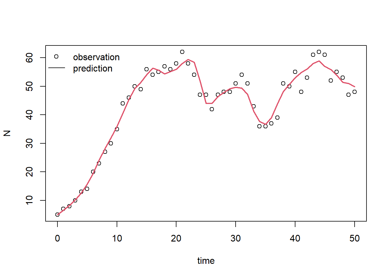
According to this plot, the model with calibrated parameter values fits the measured data much better! this should also be visible in the RMSE, so let’s confirm this by computing the RMSE (we do the same as in exercise f, but now using the calibrated parameter values):
predRMSE(p = fit$par,
         y0 = InitLogistic(),
         fn = RatesLogistic,
         name = "N",
         obs_values = surveyData$N,
         obs_times = surveyData$t)
## [1] 2.584874Indeed, we have reduced the RMSE to a value ca 2.58 via calibration. Thus, the calibrated model now fits the data (that was used for calibration) much better!
No: the model is now evaluated on the same data that was used for calibration. This should definitely not be done! The data used in calibration and evaluation should be independent! Without independent datasets, the risk of overfitting increases, and therefore we run the risk of falsely believing we have a very good explanatory model whereas in fact we have not. Here, the RMSE computed is only indicating how good the model was fitted to the calibration data! If we were to properly perform model evaluation, we would need 2 independent datasets (independent here could mean that the datasets could be from different sites, or from different time periods).
Solutions as R script
Download here the code as shown on this page in a separate .r file.